3D Multi-parametric Breast MRI Segmentation Using Hierarchical Support Vector Machine with Coil Sensitivity Correction

Rationale and Objectives

The goal of the study is to develop a technique to achieve accurate volumetric breast tissue segmentation using magnetic resonance imaging (MRI) data. This segmentation can be useful to aid in the diagnosis of breast cancers and to assess breast cancer risk based on breast density. Tissue segmentation is also essential for development of acoustic and thermal models used in magnetic resonance guided high-intensity focused ultrasound treatment of breast lesions.

Materials and Methods

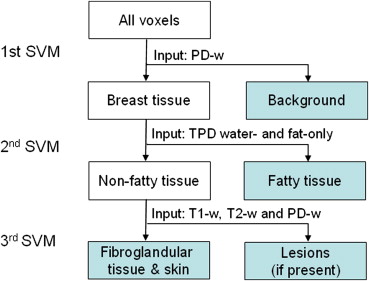
In addition to commonly used T1-, T2-, and proton density–weighted images, three-point Dixon water- and fat-only images were also included as part of the multiparametric inputs to a tissue segmentation algorithm using a hierarchical support vector machine (SVM). The effectiveness of a variety of preprocessing schemes was evaluated through two in vivo datasets. The performance of the hierarchical SVM was investigated and compared to the conventional classification algorithms—conventional SVM and fuzzy C-mean (FCM).

Results

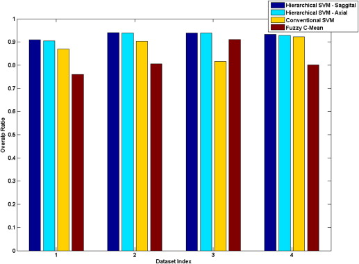
The need for co-registration, zero-filled interpolation, coil sensitivity correction, and optimal SNR reconstruction before the final stage classification was demonstrated. The overlap ratios of the hierarchical SVM, conventional SVM and FCM were 93.25%–94.08%, 81.68–92.28%, and 75.96%–91.02%, respectively. Classification outputs from in vivo experiments showed that the presented methodology is consistent and outperforms other algorithms.

Conclusion

The presented hierarchical SVM-based technique showed promising results in automatically segmenting breast tissues into fat, fibroglandular tissue, skin, and lesions. The results provide evidence that both the multiparametric breast MRI inputs and the preprocessing procedures contribute to the high accuracy of tissue classification.

Introduction

Breast magnetic resonance imaging (MRI) has become a very useful imaging modality for breast cancer screening and diagnosis . It has been shown that 17%–34 % of cancer foci visible on breast MRI are not detected by mammography . Not only does breast MRI offer higher sensitivity for detection of breast cancer than x-ray mammography, ultrasound, clinical examination, or any combination of these, it also has a superior ability to delineate fatty and fibroglandular tissue .

Although lesions can be detected by visual inspection of breast MRI images, including dynamic contrast-enhanced (DCE) studies, there is evidence that quantitative measurements of different structures in the breast with and without contrast can assist not only in the detection of abnormal tissues, but also in the discrimination between fibroadenomas, cysts, and various types of malignancies . In an attempt to improve the performance of breast computer-aided diagnosis systems that are designed to supplement visual inspection and interpretation of breast MRI, methods for fully and semiautomatic segmentation of lesion mass based on DCE-MRIs have been developed . Efforts have also been made to discriminate between benign and malignant lesions using quantitative morphological and feature analyses . In addition to automatic lesion detection and discrimination, breast tissue segmentation could also be used to determine the percentage of fibroglandular tissue present in the breast, which is directly linked to breast parenchymal patterns , where the parenchymal pattern characterization parameters are taken as risk factors of developing breast cancer .

Get Radiology Tree app to read full this article<

Materials and methods

Subjects and Image Acquisition

Get Radiology Tree app to read full this article<

Preprocessing

Get Radiology Tree app to read full this article<

Co-registration

Get Radiology Tree app to read full this article<

ZFI

Get Radiology Tree app to read full this article<

Three-point Dixon reconstruction

Get Radiology Tree app to read full this article<

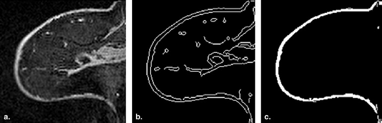
Skin extraction

Get Radiology Tree app to read full this article<

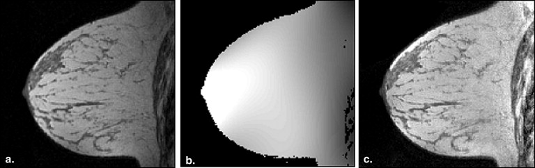
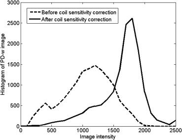
Coil sensitivity estimation

Get Radiology Tree app to read full this article<

Optimal SNR reconstruction

Get Radiology Tree app to read full this article<

Iopt(r)=R(r)Ψ−1ST(r)S(r)Ψ−1ST(r) I

(

)

(

)

−

(

)

(

)

−

(

)

where r denotes the position in the image space; R(r)=[R1(r),R2(r),…,RL(r)] R

(

)

[

(

)

(

)

…

(

)

] is the row vector of coil images; S(r)=[S1(r),S2(r),…,SL(r)] S

(

)

[

(

)

(

)

…

(

)

] is the row vector of coil sensitivities estimated from above step; and Ψ Ψ is an L by L matrix that describes the coupling and noise correlations between the coil elements. The noise matrix was assumed to be an identity matrix in the actual calculation for simplicity, and it was shown by Roemer et al that there was only a 10% SNR loss when assuming there is no noise correlation.

Get Radiology Tree app to read full this article<

Tissue Segmentation Using Hierarchical SVM

Get Radiology Tree app to read full this article<

Statistical Analysis

Get Radiology Tree app to read full this article<

Results

Get Radiology Tree app to read full this article<

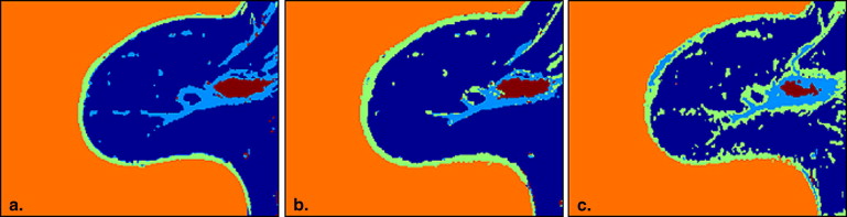
Table 1

Overlap Ratios of Various Algorithms with Radiologist’s Manual Classification as Ground Truth

Overlap Ratio h-SVM (Sagittal), % h-SVM (Axial), % c-SVM, % FCM, % h-SVM without CSC, % h-SVM without ZFI, % h-SVM without Co-registration, % Dataset 1 90.94 90.47 86.97 75.96 82.09 90.69 88.81 Dataset 2 94.08 93.92 90.30 80.58 83.42 94.50 93.67 Dataset 3 93.90 93.90 81.68 91.02 95.45 94.41 95.38 Dataset 4 93.25 92.79 92.28 80.06 81.39 92.76 81.12

Hierarchical support vector machine (h-SVM) offers highest overlap ratio than the conventional SVM (c-SVM) and the FCM algorithm. Three preprocessing steps: coil sensitivity correction (CSC), zero-filled interpolation (ZFI), and co-registration are also evaluated.

Get Radiology Tree app to read full this article<

Table 2a

Individual Tissue Type Analysis of Dataset 1 Segmentation: Correctly Classified, Incorrectly Classified, and Overlap Ratios of Hierarchical SVM for Individual Tissue Type, Comparing to the Manual Classification from Radiologist 1

Hierarchical SVM Fat Fibroglandular Skin Lesion Air Overlap Ratio, % Radiologist Fat3877 165 45 4 116 92.16 Fibroglandular 222467 17 2 1 65.87 Skin 8 37180 2 91 56.60 Lesion 0 8 08 0 50.00 Air 6 30 14 03401 98.55

References

1. Sinha S., Sinha U.: Recent advances in breast MRI and MRS. NMR Biomed 2009; 22: pp. 3-16.
2. Weatherall P.T., Evans G.F., Metzger G.J., et. al.: MRI vs. histologic measurement of breast cancer following chemotherapy: comparison with x-ray mammography and palpation. J Magn Reson Imaging 2001; 13: pp. 868-875.
3. Lee N.A., Rusinek H., Weinreb J., et. al.: Fatty and fibroglandular tissue volumes in the breasts of women 20–83 years old: comparison of X-ray mammography and computer-assisted MR imaging. AJR Am J Roentgenol 1997; 168: pp. 501-506.
4. Bhooshan N., Giger M.L., Jansen S.A., et. al.: Cancerous breast lesions on dynamic contrast-enhanced MR images: computerized characterization for image-based prognostic markers. Radiology 2010; 254: pp. 680-690.
5. Ertas G., Gulcur H.O., Osman O., et. al.: Breast MR segmentation and lesion detection with cellular neural networks and 3D template matching. Comput Biol Med 2008; 38: pp. 116-126.
6. Ertas G., Gulcur H.O., Tunaci M.: Improved lesion detection in MR mammography: three-dimensional segmentation, moving voxel sampling, and normalized maximum intensity-time ratio entropy. Acad Radiol 2007; 14: pp. 151-161.
7. Gilhuijs K.G., Giger M.L., Bick U.: Computerized analysis of breast lesions in three dimensions using dynamic magnetic-resonance imaging. Med Phys 1998; 25: pp. 1647-1654.
8. Nie K., Chen J.H., Yu H.J., et. al.: Quantitative analysis of lesion morphology and texture features for diagnostic prediction in breast MRI. Acad Radiol 2008; 15: pp. 1513-1525.
9. Nie K., Chen J.H., Chan S., et. al.: Development of a quantitative method for analysis of breast density based on three-dimensional breast MRI. Med Phys 2008; 35: pp. 5253-5262.
10. Lin M., Chan S., Chen J.H., et. al.: A new bias field correction method combining N3 and FCM for improved segmentation of breast density on MRI. Med Phys 2011; 38: pp. 5-14.
11. Kuroda K., Oshio K., Mulkern R.V., et. al.: Optimization of chemical shift selective suppression of fat. Magn Reson Med 1998; 40: pp. 505-510.
12. Jacobs M.A., Barker P.B., Bluemke D.A., et. al.: Benign and malignant breast lesions: diagnosis with multiparametric MR imaging. Radiology 2003; 229: pp. 225-232.
13. Wang CM, Mai XX, Lin GC, et al. Classification for breast MRI using support vector machine. Proceedings of the 2008 IEEE 8th International Conference on Computer and Information Technology 2008:362–367.
14. Heywang S.H., Bassermann R., Fenzl G., et. al.: MRI of the breast—histopathologic correlation. Eur J Radiol 1987; 7: pp. 175-182.
15. Meyer C.R., Bland P.H., Pipe J.: Retrospective correction of intensity inhomogeneities in MRI. IEEE Trans Med Imaging 1995; 14: pp. 36-41.
16. Guillemaud R., Brady M.: Estimating the bias field of MR images. IEEE Trans Med Imaging 1997; 16: pp. 238-251.
17. Brey W.W., Narayana P.A.: Correction for intensity falloff in surface coil magnetic resonance imaging. Med Phys 1988; 15: pp. 241-245.
18. McVeigh E.R., Bronskill M.J., Henkelman R.M.: Phase and sensitivity of receiver coils in magnetic resonance imaging. Med Phys 1986; 13: pp. 806-814.
19. Bezdek J.C.: Pattern recognition with fuzzy objective function algorithms.1981.Plenum PressNew York
20. Chen W., Giger M.L., Bick U.: A fuzzy c-means (FCM)-based approach for computerized segmentation of breast lesions in dynamic contrast-enhanced MR images. Acad Radiol 2006; 13: pp. 63-72.
21. Barck K.H., Willis B., Ross J., et. al.: Viable tumor tissue detection in murine metastatic breast cancer by whole-body MRI and multispectral analysis. Magn Reson Med 2009; 62: pp. 1423-1430.
22. Yang S.C., Wang C.M., Hsu H.H., et. al.: Contrast enhancement and tissues classification of breast MRI using Kalman filter-based linear mixing method. Comput Med Imaging Graph 2009; 33: pp. 187-196.
23. Chung P.C., Wang C.M., Yang S.H., et. al.: Tissues classification for breast MRI contrast enhancement using spectral signature detection approach. IEEE International Conference on Systems, Man and Cybernetics 2006; 5: pp. 3917-3921.
24. Du Y.P., Parker D.L., Davis W.L., et. al.: Reduction of partial-volume artifacts with zero-filled interpolation in three-dimensional MR angiography. J Magn Reson Imaging 1994; 4: pp. 733-741.
25. Glover G.H., Schneider E.: Three-point Dixon technique for true water/fat decomposition with B0 inhomogeneity correction. Magn Reson Med 1991; 18: pp. 371-383.
26. Bernstein M.A., King K.F., Zhou Z.J.: Handbook of MRI pulse sequences.2004.Academic PressBoston
27. Moon-Ho Song S., Napel S., Pelc N.J., et. al.: Phase unwrapping of MR phase images using Poisson equation. IEEE Trans Image Process 1995; 4: pp. 667-676.
28. Nie K., Chang D., Chen J.H., et. al.: Impact of skin removal on quantitative measurement of breast density using MRI. Med Phys 2010; 37: pp. 227-233.
29. Canny J.: A computational approach to edge detection. IEEE Trans Pattern Anal Mach Intell 1986; 8: pp. 679-698.
30. Vemuri P., Kholmovski E.G., Parker D.L., et. al.: Coil sensitivity estimation for optimal SNR reconstruction and intensity inhomogeneity correction in phased array MR imaging. Inf Process Med Imaging 2005; 19: pp. 603-614.
31. Roemer P.B., Edelstein W.A., Hayes C.E., et. al.: The NMR phased array. Magn Reson Med 1990; 16: pp. 192-225.
32. Cortes C., Vapnik V.: Support-vector networks. Machine Learning 1995; 20: pp. 273-297.
33. Chang C.C., Lin C.J.: LIBSVM: a library for support vector machine. ACM Trans Intell Syst Technol 2011; 2: pp. 1-27.
34. Casasent D., Wang Y.C.: A hierarchical classifier using new support vector machines for automatic target recognition. Neural Netw 2005; 18: pp. 541-548.