3D Shape Analysis of the Supraspinatus Muscle

Rationale and Objectives

Rotator cuff disorders are prevalent and can cause pain and reduced range of motion and strength. Accurate, noninvasive diagnosis of rotator cuff disorders is therefore important. In this work, we study the relationship between several three-dimensional (3D) shape measurements of the supraspinatus and its pathologic conditions. The objective is to explore the utility of 3D shape descriptors in distinguishing supraspinatus pathologies, leading to computer-aided diagnosis of rotator cuff disorders.

Materials and Methods

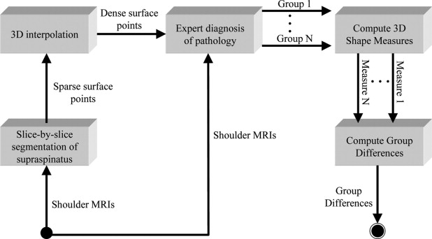
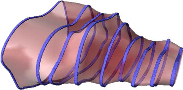
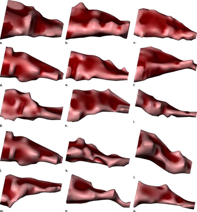
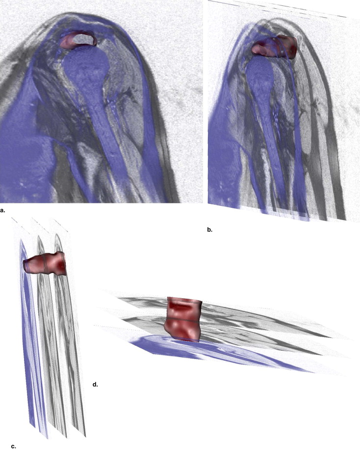
We acquired magnetic resonance images of the shoulder from 73 patients, separated into five pathology groups: normal ( ), tear ( ), tear and atrophy ( ), tear and retraction ( ), and tear and atrophy and retraction ( ). We segmented the 3D surface of the supraspinatus from each magnetic resonance image, and computed 11 3D shape characteristics for each. We performed an analysis of variance (ANOVA) test for each measurement to test the null hypothesis that the means of the pathology groups were equal. The most promising of the measurements, as determined by the ANOVA test, were used to train a support vector machine classifier to automatically assign new supraspinata to the correct pathology groups.

Results

The ANOVA test results rejected the null hypothesis ( p < .0045) for 7 of our 11 measurements. Highlights of the results from the support vector machine classifier were 79% accuracy in distinguishing normals from abnormals, and 82% accuracy in distinguishing atrophy from retraction, our main clinical motivation. These scores were tabulated based on leave-one-out cross-validation.

Conclusion

From the results, we draw the conclusion that 3D shape analysis may be helpful in the diagnosis of rotator cuff disorders, but further investigation is required to develop a 3D shape descriptor that yields ideal pathology group separation. The results of this study suggest several promising avenues of future research to meet this goal.

The rotator cuff comprises several muscles and tendons that stabilize the shoulder, including the supraspinatus ( Fig 1 ). Disorders of the rotator cuff are prevalent; incidence of disorder has been found to be 34% of asymptomatic individuals in a study where diagnosis was performed on magnetic resonance images (MRI) ( ), and 30% of individuals older than 60 years of age in a cadaveric study ( ). Symptoms of rotator cuff disorder can be debilitating, including pain, weakness, and limited range of motion, especially for overhead work ( ). Disorders of the supraspinatus muscle may involve tearing, which can lead to muscle retraction, atrophy, or both ( ). It is important to be able to distinguish between retraction and atrophy because retraction is a condition that is repairable by pulling the muscle forward in surgery, whereas atrophy is a condition uncorrectable by surgery. Because both of these conditions result in a reduction of the apparent size of the muscle and therefore are difficult to distinguish by size alone, we are motivated to investigate the utility of analyzing the 3D shape of the supraspinatus to discover shape characterizations that may assist the physician in distinguishing between these groups.

Open full size image

Figure 1

Diagram of shoulder anatomy indicating the location of the supraspinatus (posterior view). Adapted from Grey’s Anatomy ( ).

Get Radiology Tree app to read full this article<

Materials and methods

Get Radiology Tree app to read full this article<

Table 1

Description of the Pathology Groups

Abbreviation Number of Patients Pathology Group Normal: No pathology N 14 Abnormal: T, TA, TR, TAR A 59 Abnormal subgroups Tear: Full/partial tear T 20 Tear + atrophy TA 13 Tear + retraction TR 15 Tear + atrophy + retraction TAR 11

Get Radiology Tree app to read full this article<

Table 2

Descriptions of the measurements taken, with their associated measurement numbers used in this article

Number Description of Measurement 1 Eigenvalue ratio λ 1 /λ 2 2 Eigenvalue ratio λ 1 /λ 3 3 Eigenvalue ratio λ 2 /λ 3 4 Mean of distances to centroid (cm) 5 Standard deviation of distances to centroid (cm) 6 3D moment J 1 7 3D moment J 2 8 3D moment J 3 9 Surface area (cm 2 ) 10 Volume (cm 3 ) 11 Surface area/volume (1/cm)

Get Radiology Tree app to read full this article<

Ratios of Eigenvalues (Three Measures)

Get Radiology Tree app to read full this article<

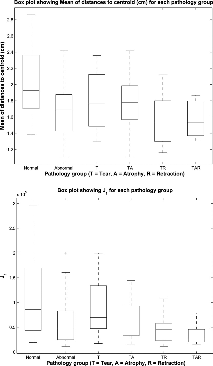
Mean and Standard Deviation of Distances to Centroid (Two Measures)

Get Radiology Tree app to read full this article<

3D Moment Invariants (Three Measures)

Get Radiology Tree app to read full this article<

J1=μ200+μ020+μ002 J

200

020

002

J2=μ200μ020+μ200μ002+μ020μ002−μ2110−μ2101−μ2011 J

200

020

200

002

020

002

−

110

−

101

−

011

J3=μ200μ020μ002+2μ110μ101μ011−μ002μ2110−μ020μ2101−μ200μ2011, J

200

020

002

110

101

011

−

002

110

−

020

101

−

200

011

where μ pqr is given by

μpqr=∑x∑y∑z(x−x¯)p(y−y¯)q(z−z¯)rf(x,y,z), μ

∑

(

−

)

(

−

)

(

−

)

(

f is given by

f(x,y,z)={1if(x,y,z)isasurfacepoint0otherwise f

(

)

{

(

)

surface

point

otherwise

x¯ x

¯ , y¯ y

¯ , z¯ z

¯ are given by

x¯=m100/m000 x

100

000

y¯=m010/m000 y

010

000

z¯=m001/m000, z

001

000

and m pqr is given by

mpqr=∑x∑y∑zxpyqzrf(x,y,z). m

∑

(

)

Get Radiology Tree app to read full this article<

Surface Area, Volume, and Their Ratios (Three Measures)

Get Radiology Tree app to read full this article<

Results

Get Radiology Tree app to read full this article<

Table 3

Mean ± standard deviation values of each of the measurements for each of the groups

N T TA TR TAR 1 2.4 ± 1.2 2.6 ± 0.90 4.0 ± 2.4 3.5 ± 1.4 3.0 ± 2.1 2 5.7 ± 2.5 6.7 ± 2.3 10 ± 5.7 7.6 ± 2.6 7.4 ± 3.3 3 2.5 ± 0.60 2.6 ± 0.69 2.7 ± 0.75 2.5 ± 0.85 3.0 ± 1.5 4 2.0 ± 0.44 1.8 ± 0.32 1.8 ± 0.34 1.6 ± 0.29 1.6 ± 0.22 5 0.65 ± 0.22 0.66 ± 0.13 0.66 ± 0.11 0.56 ± 0.13 0.6 ± 0.17 6 10.2 × 10 5 ± 9.1 × 10 4 8.7 × 10 4 ± 5.2 × 10 4 6.5 × 10 4 ± 4.2 × 10 2 4.5 × 10 4 ± 2.8 × 10 4 3.7 × 10 4 ± 2.2 × 10 4 7 5.3 × 10 9 ± 6.4 × 10 9 2.7 × 10 9 ± 2.8 × 10 9 1.5 × 10 9 ± 1.9 × 10 9 6.8 × 10 8 ± 7.3 × 10 8 4.6 × 10 8 ± 5.5 × 10 8 8 7.6 × 10 13 ± 1.1 × 10 14 2.6 × 10 13 ± 3.7 × 10 13 1.3 × 10 13 ± 2.2 × 10 13 3.2 × 10 12 ± 4.5 × 10 12 1.7 × 10 12 ± 2.8 × 10 12 9 60 ± 24 49 ± 18 45 ± 22 34 ± 7.6 34 ± 12 10 23 ± 13 15 ± 8.3 15 ± 10 9.1 ± 2.8 7.1 ± 4.7 11 2.8 ± 0.56 3.5 ± 0.80 4.8 ± 1.7 4.1 ± 1.3 5.1 ± 0.89

Please refer to Tables 1 and 2 for the meanings of the column and row labels, respectively.

Table 4

p Values resulting from a one-way analysis of variance test for each measurement, testing the null hypothesis that the means of the measurements of all of the pathology groups are the same

p Value Mean of distances to centroid (cm) .0039 3D moment J 1 .0014 3D moment J 2 .0018 3D moment J 3 .0027 Surface area (cm 2 ) .0010 Volume (cm 3 ) .000041 Surface area/volume (1/cm) .0000034

Only p values leading to rejection of the null hypothesis ( p < .0045) are shown.

Get Radiology Tree app to read full this article<

Table 5

Automated Classification Results

N T TA TR A 0.79 T 0.70 TA 0.81 0.72 TR 0.79 0.44 0.82 TAR 0.76 0.73 0.50 0.73

Each cell shows the accuracy (1 being perfect accuracy) of a support vector machine trained to distinguish the pathology groups corresponding to the row and column of that cell. Leave-one-out cross-validation was performed, with the results averaged over all rounds. The support vector machine was trained using shape features corresponding to the three smallest p values: surface area, volume, and the surface area to volume ratio. See Table 1 for abbreviations.

Get Radiology Tree app to read full this article<

Discussion

Get Radiology Tree app to read full this article<

References

1. Sher J.S., Uribe J.W., Posada A., et. al.: Abnormal findings on magnetic resonance images of asymptomatic shoulders. J Bone Joint Surg 1995; 77: pp. 10-15.
2. Lehman C., Cuomo F., Kummer F.J., et. al.: The incidence of full thickness rotator cuff tears in a large cadaveric population. Bulle Hosp Joint Dis 1995; 54: pp. 30-31.
3. Ellman H., Hanker G., Bayer M.: Repair of the rotator cuff. J Bone Joint Surg 1986; 68: pp. 1136-1144.
4. Fuchs S., Chylarecki C., Langenbrinck A.: Incidence and symptoms of clinically manifest rotator cuff lesions. A Int J Sports Med 1999; 20: pp. 201-205.
5. Gartsman G.M., Khan M., Hammerman S.M.: Arthroscopic repair of full thickness tears of the rotator cuff. J Bone Joint Surg Am 1998; 80: pp. 832-840.
6. Halder A.M., O’Driscoll S.W., Heers G., et. al.: Biomechanical comparison of effects of supraspinatus tendon detachments, tendon defects, and muscle retractions. J Bone Joint Surg 2002; 84-A: pp. 780-785.
7. Itoi E., Hsu H.-C., Carmichael S.W., et. al.: Morphology of the torn rotator cuff. J Anat 1995; 186: pp. 429-434.
8. Robertson P.L., Schweitzer M.E., Mitchell D.G., et. al.: Rotator cuff disorders: Interobserver and intraobserver variation in diagnosis with MR imaging. Radiology 1995; 194: pp. 831-835.
9. Thomazeau H., Rolland Y., Lucas C., et. al.: Atrophy of the supraspinatus belly. Acta Orthop Scand 1996; 67: pp. 264-268.
10. Gray H.: Anatomy of the human body.1918.Lea and FebigerPhiladelphia, Pa:
11. Fuchs B., Weishaupt D., Zanetti M., et. al.: Fatty degeneration of the muscles of the rotator cuff: Assessment by computed tomography versus magnetic resonance imaging. J Shoulder Elbow Surg 1999; 8: pp. 599-605.
12. Zanetti M., Gerber C., Hodler J.: Quantitative assessment of the muscles of the rotator cuff with magnetic resonance imaging. Investig Radiol 1998; 33: pp. 163-170.
13. Bachmann G.F., Melzer C., Heinrichs C.M., et. al.: Diagnosis of rotator cuff lesions: comparison of US and MRI on 38 joint specimens. Eur Radiol 1997; 7: pp. 192-197.
14. Quinn S.F., Sheley R.C., Demlow T.A., et. al.: Rotator cuff tendon tears: Evaluation with fat-suppressed MR imaging with arthroscopic correlation in 100 patients. Radiology 1995; 195: pp. 497-500.
15. Swen W.A.A., Jacobs J.W.G., Algra P.R., et. al.: Sonography and magnetic resonance imaging equivalent for the assessment of full-thickness rotator cuff tears. Arthritis Rheum 1999; 42: pp. 2231-2238.
16. Zlatkin M., Iannotti J., Roberts M., et. al.: Rotator cuff tears: Diagnostic performance of MR imaging. Radiology 1989; 172: pp. 223-229.
17. Mortensen M.E.: Geometric modeling.1985.John Wiley & Sons, IncNew York
18. Lehtinen J.T., Tingart M.J., Apreleva M., et. al.: Practical assessment of rotator cuff muscle volumes using shoulder MI. Acta Orthop Scand 2003; 74: pp. 722-729.
19. Turk G., O’Brien J.F.: Shape transformation using variational implicit functions. Proc ACM SIGGRAPH 1999; pp. 335-342.
20. Jolliffe I.T.: Principal components analysis.1986.Springer-VerlagNew York
21. Sadjadi F.A., Hall E.L.: Three-dimensional moment invariants. IEEE PAMI 1980; 2: pp. 127-136.
22. Lorensen W.E., Cline H.E.: Marching cubes: A high resolution 3D surface construction algorithm.1987.ACM PressNew York:
23. Abdi H.: Bonferroni and Sidak corrections for multiple comparisons.Salkind N.J.Encyclopedia of measurement and statistics.2007.SageThousand Oaks, Calif:
24. Fradkin D., Muchnik I.: Support vector machines for classification.Abello J.Carmode G.Discrete methods in epidemiology.2006.pp. 13-20.

3D Shape Analysis of the Supraspinatus Muscle

Rationale and Objectives

Materials and Methods

Results

Conclusion

Materials and methods

Ratios of Eigenvalues (Three Measures)

Mean and Standard Deviation of Distances to Centroid (Two Measures)

3D Moment Invariants (Three Measures)

Surface Area, Volume, and Their Ratios (Three Measures)

Results

Discussion

References

Further Reading

A Computer-Based Radiology Simulator as a Learning Tool to Help Prepare First-Year Residents for Being On Call

A Review of Research Into the Development of Radiologic Expertise Implications for Computer-Based Training

A Validation Framework for Brain Tumor Segmentation