A Dynamic Graph Cuts Method with Integrated Multiple Feature Maps for Segmenting Kidneys in 2D Ultrasound Images

Rationale and Objectives

Automatic segmentation of kidneys in ultrasound (US) images remains a challenging task because of high speckle noise, low contrast, and large appearance variations of kidneys in US images. Because texture features may improve the US image segmentation performance, we propose a novel graph cuts method to segment kidney in US images by integrating image intensity information and texture feature maps.

Materials and Methods

We develop a new graph cuts-based method to segment kidney US images by integrating original image intensity information and texture feature maps extracted using Gabor filters. To handle large appearance variation within kidney images and improve computational efficiency, we build a graph of image pixels close to kidney boundary instead of building a graph of the whole image. To make the kidney segmentation robust to weak boundaries, we adopt localized regional information to measure similarity between image pixels for computing edge weights to build the graph of image pixels. The localized graph is dynamically updated and the graph cuts-based segmentation iteratively progresses until convergence. Our method has been evaluated based on kidney US images of 85 subjects. The imaging data of 20 randomly selected subjects were used as training data to tune parameters of the image segmentation method, and the remaining data were used as testing data for validation.

Results

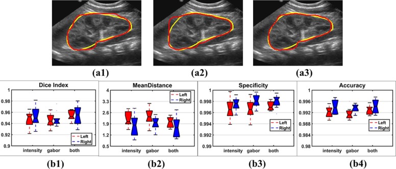
Experiment results demonstrated that the proposed method obtained promising segmentation results for bilateral kidneys (average Dice index = 0.9446, average mean distance = 2.2551, average specificity = 0.9971, average accuracy = 0.9919), better than other methods under comparison ( P < .05, paired Wilcoxon rank sum tests).

Conclusions

The proposed method achieved promising performance for segmenting kidneys in two-dimensional US images, better than segmentation methods built on any single channel of image information. This method will facilitate extraction of kidney characteristics that may predict important clinical outcomes such as progression of chronic kidney disease.

Introduction

Ultrasound (US) imaging has been widely used to examine kidneys for structural abnormalities and to measure kidney anatomic features such as renal parenchymal area that have been associated with development of end stage renal disease . utomatic segmentation of US images of kidneys will facilitate extraction and quantification of anatomic features such as renal parenchymal area and kidney echogenicity, which currently are measured manually. However, automatic segmentation of kidneys in (two-dimensional) 2D US images remains a challenging task due to high speckle noise, low contrast between foreground and background, weak boundaries, and large appearance variations of kidneys in 2D US images . A

A variety of automatic methods have been developed for segmenting kidneys in 2D US images, including active contour model (ACM)-based methods , atlas-based methods , Markov random field-based methods , watershed-based methods , machine learning-based methods , and deep learning methods . Among them, the ACM-based method is appealing because of its robustness to imaging noise, weak boundaries, and large appearance variation within kidneys. However, the existing ACM-based image segmentation methods typically adopt gradient descent flow-based optimization techniques, which often get stuck at local minima . Such a limitation can be overcome by graph cuts (GC) techniques . Particularly, GC techniques model the image segmentation task as an image labeling problem on a graph . The GC techniques can be integrated with the ACM-based methods by transforming the minimization problem of the ACM methods into a minimum-cut problem of a graph . However, speckle noise and low contrast of US images might degrade the segmentation performance if the US images are directly used as input to the segmentation algorithms.

Get Radiology Tree app to read full this article<

Materials and Methods

Get Radiology Tree app to read full this article<

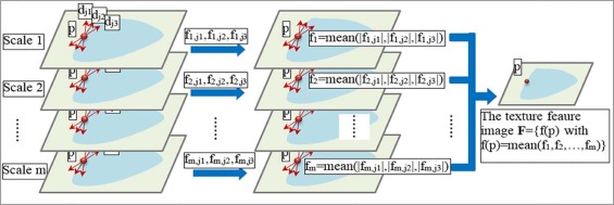
Texture Feature Map Extraction

Get Radiology Tree app to read full this article<

{g=12πσxσyexp(−(x′σ2x+y′σ2y))exp(i(2πx′λ))x′=xcosθ+ysinθ,y′=−xsinθ+ycosθ, {

(

−

(

′

)

(

′

)

′

xcosθ

ysinθ

′

−

xsinθ

ycosθ

where σ x and σ y are standard deviations of the Gaussian functions along axis x and axis y respectively, θ is the direction of the Gabor filter, wavelength λ is the frequency factor, and the frequency ω=2πλ ω

λ . A Gabor filter with a small λ captures image information of high frequency and small scale, whereas a Gabor filter with a big λ captures image information of low frequency and big scale. Gabor filters in different scales, and directions can be integrated to capture multiscale image information .

Get Radiology Tree app to read full this article<

gi=argmaxj=1,…,n|fi,j(p)|,i=1,…,m, g

argmax

…

(

)

…

where the dominant direction at scale i has the maximum absolute value, ∣∣fi,gi(p)∣∣ |

(

)

| , among all directions. For every direction, we then compute the number of scales at which the direction under consideration is the dominant direction.

Dj=∑mi=1δ(|fi,j(p)|−∣∣fi,gi(p)∣∣),j=1,…,n D

∑

(

)

−

(

)

…

where function δ (∙) is 1 at zero and 0 otherwise. Finally, we identify dominant directions across all scales as

Ω={j|Dj≥0.5⋅maxj=1,..,nDj}, Ω

{

≥

0.5

⋅

max

}

where dominant directions are identified as those with filtering responses greater than half of the maximal response values to balance robustness and redundancy of the dominant directions.

Get Radiology Tree app to read full this article<

f(p)=1m∑mi=1∑j∈Ω|fi,j(p)|. f

(

)

∑

∈

(

)

Get Radiology Tree app to read full this article<

Dynamic GC-Based Image Segmentation with Integrated Multiple Feature Maps

Get Radiology Tree app to read full this article<

w(p,q)=α⋅wp(p,q)+(1−α)⋅wr(p,q), w

(

)

⋅

(

)

(

−

)

⋅

(

)

wp(p,q)=exp(−1N∑Ni=1(Ii(p)−Ii(q))2σ),wr(p,q)=exp(−(1/(1N∑Ni=1Ki(p,q)))σ), w

(

)

(

−

∑

(

)

−

(

)

(

)

(

−

(

∑

(

)

where p and q are adjacent pixels, wp(p,q) w

(

) and wr(p,q) w

(

) are image similarity measures based on pixel information and regional information respectively, α is a trade-off parameter between the two terms, Ii(p) I

(

) and Ii(q) I

(

) are image intensity value of p and q for the i th feature map, Ki(p,q) K

(

) is an image difference measure based on regional information, σ is a parameter, and i = 1, 2 corresponding to the original US image intensity and the Gabor feature map respectively. The numerator terms in both wp(p,q) w

(

) and wr(p,q) w

(

) are normalized to [0,1]. Particularly, Ki(p,q) K

(

) is defined as

Ki(p,q)=min(lp,lq)∈{(S,T),(T,S),(S,S)or(T,T)}(Ii(p)−flpi(p))2+(Ii(q)−flqi(q))2, K

(

)

min

(

)

∈

{

(

)

(

)

(

)

(

)

}

(

)

−

(

)

(

)

−

(

)

where Ii(p) I

(

) and Ii(q) I

(

) are image intensity value of p and q for the i th feature map, fSi(p) f

(

) , fTi(p) f

(

) , fSi(q) f

(

) , fTi(q) f

(

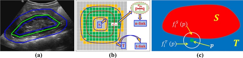
) are intensity mean of pixels of a small neighborhood of p and q corresponding to segments S and T , respectively, as illustrated in Figure 3 c, and lp∈{S,T} l

∈

{

} and lq∈{S,T} l

∈

{

} are possible segmentation labels of p and q to be updated according to the minimal value computed by Equation 7 . Particularly, Ki(p,q) K

(

) measures differences between image intensity values of pixels and mean image intensity values of their corresponding optimal segmentation results. However, if the optimal segmentation labels of p and q are the same, we set Ki(p,q)=max(u,v)∈(V,V)Ki(u,v) K

(

)

max

(

)

∈

(

)

(

) so that they will not be separated into different segments.

Get Radiology Tree app to read full this article<

Segmentation Performance Evaluation and Parameter Optimization

Get Radiology Tree app to read full this article<

Results

Optimization of the Parameters

Get Radiology Tree app to read full this article<

Experiments on Single and Multiple Feature Maps

Get Radiology Tree app to read full this article<

Experiments on Different Settings of Image Similarity Measures

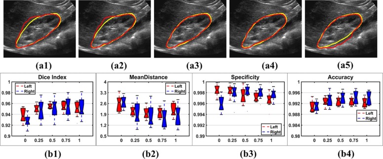
Get Radiology Tree app to read full this article<

Experiments on Different Initializations

Get Radiology Tree app to read full this article<

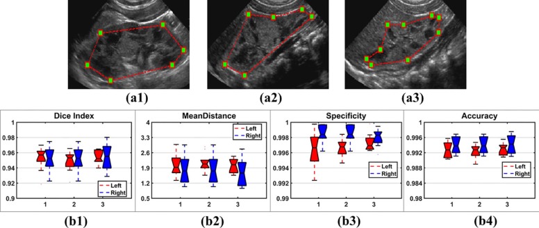
Table 1

Intraclass Correlation Coefficients for Three Different Initializations

Dice Index Mean Distance Specificity Accuracy 0.8531 0.8329 0.8549 0.8691

Get Radiology Tree app to read full this article<

Experiments on Different Narrowbands

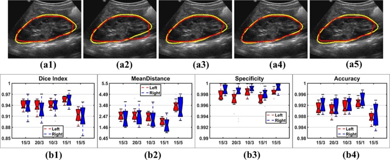
Get Radiology Tree app to read full this article<

Comparison with Alternative Methods

Get Radiology Tree app to read full this article<

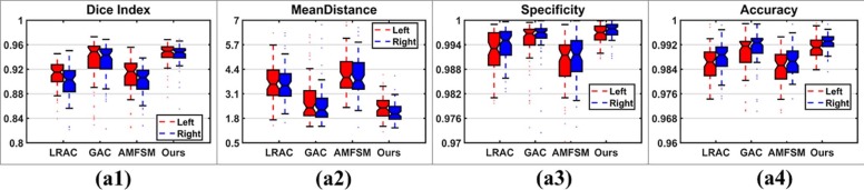
Table 2

Segmentation Accuracy Measures of Results Obtained by Different Methods (Paired Wilcoxon Rank Sum Tests Were Adopted to Compare the Proposed Method with the Alternatives)

Dice Index Mean Distance Mean Std Median_P_ value Mean Std Median_P_ value LRAC 0.9051 0.0257 0.9093 5.12e–23 3.6527 0.9810 3.5612 8.14e–23 GAC 0.9315 0.0374 0.9465 3.99e–04 2.9888 2.0283 2.2896 1.02e–04 AMFSM 0.9024 0.0388 0.9118 2.04e–22 4.1275 1.1435 3.9175 1.51e–22 Proposed 0.9446 0.0179 0.9489 2.2551 0.5783 2.1941

Specificity Accuracy Mean Std Median_P_ value Mean Std Median_P_ value LRAC 0.9932 0.0048 0.9941 3.73e–13 0.9868 0.0053 0.9877 1.02e–22 GAC 0.9945 0.0087 0.9969 1.24e–04 0.9894 0.0085 0.9918 1.00e–03 AMFSM 0.9901 0.0065 0.9915 6.33e–21 0.9854 0.0054 0.9858 1.75e–22 Proposed 0.9971 0.0022 0.9976 0.9919 0.0031 0.9924

AMFSM, adaptive multifeature segmentation model; GAC, geodesic active contours; LRAC, localizing region-based active contours; Std, standard deviation.

Get Radiology Tree app to read full this article<

Discussion and Conclusions

Get Radiology Tree app to read full this article<

References

1. Gao J., Perlman A., Kalache S., et. al.: Multiparametric quantitative ultrasound imaging in assessment of chronic kidney disease. J Ultrasound Med 2017; 36: pp. 2245-2256.
2. Cost G.A., Merguerian P.A., Cheerasarn S.P., et. al.: Sonographic renal parenchymal and pelvicaliceal areas: new quantitative parameters for renal sonographic followup. J Urology 1996; 156: pp. 725-729.
3. Pulido J.E., Furth S.L., Zderic S.A., et. al.: Renal parenchymal area and risk of ESRD in boys with posterior urethral valves. Clin J Am Soc Nephrol 2014; 9: pp. 499-505.
4. Noble J.A., Boukerroui D.: Ultrasound image segmentation: a survey. IEEE Trans Med Imaging 2006; 25: pp. 987-1010.
5. Song Y.H., Wang H.X., Liu Y., et. al.: An improved level set method for segmentation of renal parenchymal area from ultrasound images. J Med Imaging Health Inform 2016; 5: pp. 1533-1536.
6. Yang F., Qin W.J., Xie Y.Q., et. al.: A shape optimized framework for kidney segmentation in ultrasound images using NLTV denoising and DRLSE. Biomed Eng 2012; 11: pp. 1-13.
7. Marsousi M., Plataniotis K.N., Stergiopoulos S.: Atlas-based organ segmentation in 3D ultrasound images and its application in automated kidney segmentation.Processing of the 37th International Conference of the IEEE in Engineering in Medicine and Biology Society (EMBC).2015.pp. 2001-2005.
8. Martin-Fernandez M., Alberola-Lopez C.: An approach for contour detection of human kidneys from ultrasound images using Markov random fields and active contours. Med Image Anal 2005; 9: pp. 1-23.
9. Tamilselvi P.R., Thangaraj P.: A modified watershed segmentation method to segment renal calculi in ultrasound kidney images. J Intell Manuf 2012; 8: pp. 46-61.
10. Ardon R., Cuingnet R., Bacchuwar K., et. al.: Fast kidney detection and segmentation with learned kernel convolution and model deformation in 3D ultrasound image.Processing of 12th IEEE International Symposium on Biomedical Imaging (ISBI).2015.pp. 268-271.
11. Ravishankar H., Venkataramani R., Thiruvenkadam S., et. al.: Learning and incorporating shape models for semantic segmentation.International conference on Medical Image Computing and Computer-Assisted Intervention, MICCAI.2017.pp. 203-211.
12. Ronneberger O., Fischer P., Brox T.: U-Net: convolutional network for biomedical image segmentation.International Conference on Medical Image Computing and Computer-Assisted Intervention, MICCAI.2015. 9351:234-41
13. Bae E., Tai X.C.: Graph Cuts for the Multiphase Mumford-Shah Model Using Piecewise Constant Level Set Methods. UCLA Applied Mathematics2008. CAM-report-08-36
14. Tao W.B.: Iterative narrowband based graph cuts optimization for geodesic active contours with region forces (GACWRF). IEEE Trans Image Process 2012; 21: pp. 284-296.
15. Liu L.M., Tao W.B., Liu J., et. al.: A variational model and graph cuts optimization for interactive foreground extraction. Signal Process 2011; 91: pp. 1210-1215.
16. Boykov Y., Kolmogorov V.: An experimental comparison of min-cut/max-flow algorithms for energy minimization in vision. IEEE Trans Pattern Anal Mach Intell 2004; 26: pp. 1124-1137.
17. Boykov Y., Veksler O., Zabih R.: Fast approximate energy minimization via graph cuts. IEEE Trans Pattern Anal Mach Intell 2001; 23: pp. 1222-1238.
18. Le T.H., Jung S.-W., Choi K.-S., et. al.: Image segmentation based on modified graph cut algorithm. Electron Lett 2010; 46: pp. 1121-1122.
19. Xu N., Ahuja N., Bansal R.: Object segmentation using graph cuts based active contours. IEEE Conf Comput Vision Pattern Recogn 2003; 2: pp. 46-53.
20. Huang Q.H., Lee S.Y., Liu L.Z., et. al.: A robust graph-based segmentation method for breast tumors in ultrasound images. Ultrasonics 2012; 52: pp. 266-275.
21. Zhang P., Liang Y.M., Chang S.J., et. al.: Kidney segmentation in CT sequences using graph cuts based active contours model and contextual continuity. Med Phys 2013; 40: pp. 081905.
22. Tian Z.Q., Liu L.Z., Zhang Z.F., et. al.: Superpixel based segmentation for 3D prostate MR images. IEEE Trans Med Imaging 2016; 35: pp. 791-801.
23. Xie J., Jiang Y.F., Tsui H.: Segmentation of kidney form ultrasound images based on texture and shape priors. IEEE Trans Med Imaging 2005; 24: pp. 45-57.
24. Faucheux C., Olivier J., Bone R., et. al.: Texture-based graph regularization process for 2D and 3D ultrasound image segmentation.19th IEEE International Conference on Image Processing.2012.pp. 2333-2336.
25. Jokar E., Pourghassem H.: Kidney segmentation in ultrasound images using curvelet transform and shape prior.2013 International Conference on Communications Systems and Network Technologies.2013.pp. 180-185.
26. Cerrolaza J.J., Safdar N., Biggs E., et. al.: Renal segmentation from 3D ultrasound via fuzzy appearance models and patient-specific alpha shapes. IEEE Trans Med Imaging 2016; 35: pp. 1-10.
27. Mehrnaz Z.Q., Jagath S.: 2D ultrasound images segmentation using graph cuts and local image features.IEEE Symposium on Computational Intelligence for Image Processing.2009.pp. 33-40.
28. Jia R., Mellon S.J., Hansjee S., et. al.: Automatic bone segmentation in ultrasound images using loca phase features and dynamic programming.2016 IEEE 13th International Symposium on Biomedical Imaging (ISBI).2016.pp. 1005-1008.
29. Hacihaliloglu L., Abugharbieh R., Hodgson A.J., et. al.: Automatic adaptive parameterization in local phase feature based bone segmentation in ultrasound. Ultrasound Med Biol 2011; 37: pp. 1689-1703.
30. Wu Q.G., Gan Y., Lin B., et. al.: An active contour model based fused texture features for image segmentation. Neurocomputing 2015; 151: pp. 1133-1141.
31. Cohen F.S., Cooper D.B.: Simple parallel hierarchical and relaxation algorithms for segmenting noncausal Markovian random fields. IEEE Trans Pattern Anal Mach Intell 1987; 9: pp. 195-219.
32. Haralick R.M., Shanmugam K., Dinstein I.: Textural features for image classification. IEEE Trans Syst Man Cybenetics 1973; 3: pp. 610-621.
33. Daugman J.G.: Uncertainty relation for resolution in space, spatial frequency, and orientation optimized by two-dimensional visual cortical filters. J Opt Soc Am A 1985; 2: pp. 1160-1169.
34. Cunha A.L., Zhou J.P., Do M.N.: The nonsubsampled contourlet transform: theory, design, and applications. IEEE Trans Image Process 2006; 15: pp. 3089-3101.
35. Malik J., Belongie S., Leung T., et. al.: Contour and texture analysis for image segmentation. Int J Comput Vision 2001; 43: pp. 7-27.
36. Sandberg B., Chan T., Vese L.: A level set and Gabor based active contour algorithm for segmenting textured images. UCLA Department of Mathematics CAM report2002.
37. Marcelja S.: Mathematical description of the responses of simple cortical cells. J Opt Soc Am 1980; 70: pp. 1297-1300.
38. Jones J.P., Palmer L.A.: An evaluation of the two-dimensional Gabor filter model of simple receptive fields in cat striate cortex. J Neurophysiol 1987; 58: pp. 1233-1258.
39. Yang J.W., Liu L.F., Jiang T.Z., et. al.: A modified Gabor filter design method for fingerprint image enhancement. Pattern Recogn Lett 2003; 24: pp. 1805-1817.
40. Boykov Y., Jolly M.: Interactive graph cuts for optimal boundary & region segmentation of objects in N-D images. IEEE Int Conf Comput Vision 2001; 1: pp. 105-112.
41. Lankton S., Tannenbaum A.: Localizing region based active contours. IEEE Trans Image Process 2008; 17: pp. 2029-2039.
42. Caselles V., Kimmel R., Sapiro G.: Geodesic active contours. Int J Comput Vision 1997; 22: pp. 61-79.
43. Dietenbeck T., Alessandrini M., Friboulet D., et. al.: Creaseg: a free software for the evaluation of image segmentation algorithms based on level set. IEEE Int Conf Image Process 2010; 119: pp. 665-668.
44. Chan T., Vese L.: Active contours without edges. IEEE Trans Image Process 2010; 10: pp. 266-277.
45. Li C.M., Kao C.Y., Core J.C., et. al.: Minimization of region-scalable fitting energy for image segmentation. IEEE Trans Image Process 2008; 17: pp. 1940-1949.
46. Bernard O., Friboulet D., Thevenaz P., et. al.: Variational B-spline level set: a linear filter approach for fast deformable model evolution. IEEE Trans Image Process 2009; 18: pp. 1179-1191.
47. Shi Y.G., Karl W.: A real-time algorithm for the approximation of level set based curve evolution. IEEE Trans Image Process 2008; 17: pp. 645-656.
48. Zhang T.T., Han J., Zhang Y., et. al.: An adaptive multi-feature segmentation model for infrared image. Optical Rev 2016; 23: pp. 220-230.
49. McGraw K.O., Wong S.P.: Forming inferences about some intraclass correlation coefficients. Psychol Methods 1996; 1: pp. 30-46.

A Dynamic Graph Cuts Method with Integrated Multiple Feature Maps for Segmenting Kidneys in 2D Ultrasound Images

Rationale and Objectives

Materials and Methods

Results

Conclusions

Introduction

Materials and Methods

Texture Feature Map Extraction

Dynamic GC-Based Image Segmentation with Integrated Multiple Feature Maps

Segmentation Performance Evaluation and Parameter Optimization

Results

Optimization of the Parameters

Experiments on Single and Multiple Feature Maps

Experiments on Different Settings of Image Similarity Measures

Experiments on Different Initializations

Experiments on Different Narrowbands

Comparison with Alternative Methods

Discussion and Conclusions

References

Further Reading

Neurometabolites Alteration in the Acute Phase of Mild Traumatic Brain Injury (mTBI)

Reinforcing the Importance and Feasibility of Implementing a Low-dose Protocol for CT-guided Biopsies

Rethinking the PGY-1 Basic Clinical Year