
Rationale and Objectives
A phantom set was devised to evaluate capability of independent component analysis (ICA) as an image filter for magnetic resonance (MR) images to segregate components.
Materials and Methods
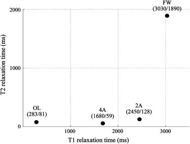
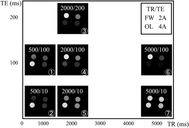
Four components (free water [FW], olive oil [OL], 2% and 4% agar gels [2A and 4A, respectively]) were arranged in a phantom set. Seven MR images were obtained with different echo time and repetition time. ICA was performed on 23 combinations of four components. A segregation rate higher than 70% was defined as effective.
Results
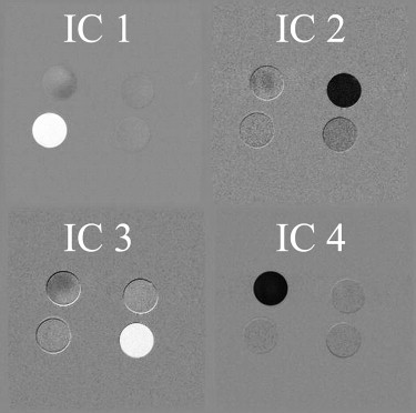
Four-component segregation was obtained in 5 of 23 combinations. The best result showed a mean of 87% across the four components. For each component, there were 20 of 23 for FW, 22 for OL, 9 for 2A, and 16 for 4A.
Conclusions
The results demonstrated ICA works as an image filter and provides new contrast images that unambiguously segregate components in MR images. For practical application, the best performance should be obtained when T 1 W, T 2 W, and proton density images are included in the dataset for ICA.
For the past decade, use of an independent component analysis (ICA) for tissue classification in magnetic resonance (MR) images has been reported . Tissues have intrinsic longitudinal and transversal relaxation times (T1 and T2, respectively) that are physically independent of each other. The ICA segregates tissues according to characteristics in a relaxation time domain, which our group has previously demonstrated with human brains . In this study, we obtained three new image contrasts as unmixed components—short T 1 components (myelin of white matter and lipids), relatively short T 1 components (intracellular water and gray matter), and long T 2 components (free water)—that were calculated from T1-weighted (T1 W), T2-weighted (T2 W), and proton density (PD) images. The results indicated potential for obtaining enhanced contrast images of gray and white matter by using ICA.
It should be noted, however, that heterogeneousness of real organs ( ) is not necessarily ideal for evaluating an image filter because it may undermine clarity of results. For rigorous evaluation, relaxation characteristics of the object should be operationally defined; therefore, a phantom set should be devised that includes different components in different spatial locations.
Get Radiology Tree app to read full this article<
Materials and methods
Get Radiology Tree app to read full this article<
MR Imaging for Calculating T 1 and T 2 Relaxation Times of the Four Components
Get Radiology Tree app to read full this article<
Get Radiology Tree app to read full this article<
T1:STI=S0{1−2exp(−TI/T1)}, T
1
:
S
T
I
=
S
0
{
1
−
2
exp
(
−
T
I
/
T
1
)
}
,
T2:STE=S0exp(−TE/T2), T
2
:
S
T
E
=
S
0
exp
(
−
T
E
/
T
2
)
,
where S TI and S TE represent the measured signal intensities for a given TI and TE, respectively, and S 0 is the signal intensity of the equilibrium state.
Get Radiology Tree app to read full this article<
ICA
Get Radiology Tree app to read full this article<
Get Radiology Tree app to read full this article<
Get Radiology Tree app to read full this article<
Segregation rate(ICkcom)(%)={∑18×18S=1(ICkcom(S)−ICbak(s))2}1/2∑4k=1{∑18×18S=1(ICkcom(S)−ICbak(S))2}1/2×100, Segregation rate
(
I
C
com
k
)
(
%
)
=
{
∑
S
=
1
18
×
18
(
I
C
c
o
m
k
(
S
)
−
I
C
b
a
k
(
s
)
)
2
}
1
/
2
∑
k
=
1
4
{
∑
S
=
1
18
×
18
(
I
C
c
o
m
k
(
S
)
−
I
C
b
a
k
(
S
)
)
2
}
1
/
2
×
100
,
where ICkcom I
C
c
o
m
k and IC bak represent average signal intensity within the original component (ie, k is the component FW, OL, 2A, or 4A, and the background, respectively) and s is the pixel number). The segregation rate above 70% was defined as effective.
Get Radiology Tree app to read full this article<
Results
Get Radiology Tree app to read full this article<
Get Radiology Tree app to read full this article<
Table 1
The Component Segregation Rate (%) after ICA
Free Water Olive Oil 2% Agar Gel 4% Agar Gel Reference number MR images IC1 IC2 IC3 IC4 IC1 IC2 IC3 IC4 IC1 IC2 IC3 IC4 IC1 IC2 IC3 IC4 1 1,2,3,4 7.073.7 3.5 15.8 1.1 0.093.6 5.382.5 4.1 1.0 12.4 42.4 7.1 14.1 36.5 2 1,2,3,576.6 3.2 1.6 18.5 0.093.6 3.7 2.8 5.6 0.0 47.6 46.8 6.4 0.8 66.4 26.4 3 1,2,3,6 0.0 7.083.7 9.388.1 3.6 3.6 4.8 2.2 68.5 9.8 19.6 16.4 47.5 1.6 34.4 4 1,2,3,776.0 3.2 4.0 16.8 0.091.9 3.6 4.5 4.8 0.8 53.6 40.8 6.5 1.6 61.3 30.6 5 1,2,4,5 6.7 1.185.6 6.7 1.192.3 3.3 3.3 41.7 1.0 29.2 28.179.1 4.4 7.7 8.8 6 1,2,4,781.1 0.0 3.2 15.8 0.0 0.096.6 3.4 24.5 46.9 2.0 26.5 10.372.2 5.2 12.4 7 1,2,5,6 1.287.2 1.2 10.588.8 3.4 4.5 3.4 0.0 23.1 46.2 30.8 1.1 12.072.8 14.1 8 1,2,6,783.3 2.2 6.7 7.8 0.092.0 4.6 3.4 16.5 1.1 52.7 29.7 15.5 1.0 67.0 16.59 1,3,4,7 7.7 9.4 1.781.2 1.0 1.095.2 2.987.5 6.7 2.9 2.9 8.384.3 4.6 2.810 1,3,5,6 10.377.9 8.8 2.9 1.7 1.7 3.393.3__71.6 10.4 11.9 6.0 5.0 3.388.3 3.3 11 1,3,5,7 15.4 0.0 22.2 62.4 1.194.3 3.4 1.1 20.9 1.176.9 1.186.2 3.4 2.3 8.012 1,3,6,7 1.475.0 16.7 6.990.5 3.2 1.6 4.8 3.2 3.277.4 16.1 1.7 1.7 3.493.1 13 1,4,5,7 8.5 69.0 18.3 4.2 1.7 0.0 6.891.5 34.8 24.6 34.8 5.879.7 5.1 11.9 3.4 14 1,5,6,7 7.5 69.2 17.8 5.6 1.1 1.1 8.089.8 35.1 17.1 41.4 6.376.7 4.4 16.7 2.2 15 2,3,4,678.0 12.2 7.3 2.4 2.9 0.0 2.994.3 6.1 6.187.9 0.0 9.1 4.5 63.6 22.716 2,3,4,7 0.0 6.485.5 8.290.7 4.6 2.8 1.9 0.9 9.4 3.885.8 1.986.4 2.9 8.7 17 2,3,5,6 9.8 1.682.0 6.6 1.893.0 1.8 3.5 68.3 1.6 11.1 19.0 1.9 1.9 5.790.6 18 2,3,6,7 7.9 1.6 9.581.0 1.793.1 3.4 1.7 68.8 1.6 18.8 10.9 3.8 1.994.2 0.0 19 2,4,5,689.2 2.7 2.7 5.4 0.0 0.0100.0 0.0 29.4 52.9 2.9 14.7 12.572.5 5.0 10.0 20 2,4,6,7 2.6 10.5 2.684.2__91.9 2.7 2.7 2.7 0.0 6.3 62.5 31.3 2.8 11.175.0 11.1 21 3,4,6,7 2.4 9.5 4.883.3 35.7 2.4 59.5 2.4 7.385.4 4.9 2.4 16.1 3.280.6 0.022 3,5,6,7 7.674.7 16.5 1.3 4.5 1.5 1.592.5 7.9 3.285.7 3.276.1 1.4 18.3 4.2 23 4,5,6,7 7.378.0 0.0 14.6 5.4 0.089.2 5.4 8.6 14.3 8.6 68.6 11.6 23.3 7.0 58.1
The numbers of magnetic resonance images correspond to those in Fig. 2 . In this table, effective (>70%) four-component segregation is indicated with a black cell effective (>70%) single-component segregation is indicated with a gray cell.
Get Radiology Tree app to read full this article<
Discussion
Get Radiology Tree app to read full this article<
Get Radiology Tree app to read full this article<
Get Radiology Tree app to read full this article<
Acknowledgments
Get Radiology Tree app to read full this article<
References
1. Bell A.J., Sejnowski T.J.: An information-maximization approach to blind separation and blind deconvolution. Neural Comput 1995; 7: pp. 1129-1159.
2. Amari S.: Natural gradient works efficiently in learning. Neural Comput 1998; 10: pp. 251-276.
3. Cardoso J.F., Laheld B.: Equivariant adaptive source separation. IEEE Trans Signal Process 1996; 45: pp. 434-444.
4. Muraki S., Nakai T., Kita Y., et. al.: An attempt for coloring multichannel MR imaging data. IEEE Trans Vis Comput Graph 2001; 7: pp. 265-274.
5. Nakai T., Muraki S., Bagarinao E., et. al.: Magnetic resonance imaging for enhancing the contrast of gray and white matter. NeuroImage 2004; 21: pp. 251-260.
6. Amato U., Larobina M., Antoniadis A., et. al.: Segmentation of magnetic resonance brain images through discriminant analysis. J Neurosci Methods 2003; 131: pp. 65-74.
7. Chen YW, Sugiki D. Segmentation of MR images using independent component analysis. In: Knowledge-Based Intelligent Information and Engineering Systems. 10th International Conference, KES 2006, Bournemouth, UK, October 9–11, 2006. Proceedings, Part II. Springer Berlin/Heidelberg, 2006; 4252:63–69.
8. Ouyang Y.C., Chen H.M., Chai J.W., et. al.: Band expansion-based over-complete independent component analysis for multispectral processing of magnetic resonance images. IEEE Trans Biomed Eng 2008; 6: pp. 1666-1677.
9. Logothetis N.K.: What we can do and what we cannot do with fMRI. Nature 2008; 453: pp. 869-878.
10. Hyvarinen A.: Fast and robust fixed-point algorithms for independent component analysis. IEEE Trans Neural Netw 1999; 10: pp. 626-634.
11. Hyvarinen A., Karhunen J., Oja E.: Independent component analysis.2001.Wiley-Interscience PublicationNew York