A Quantitative Description of the Percentage of Breast Density Measurement Using Full-field Digital Mammography

Rationale and Objectives

Breast density is a significant breast cancer risk factor that is measured from mammograms. However, uncertainty remains in both understanding its underlying physical properties as it relates to the breast and determining the optimal method for its measurement. A quantitative description of the information captured by the standard operator-assisted percentage of breast density (PD) measure was developed using full-field digital mammography (FFDM) images that were calibrated to adjust for interimage acquisition technique differences.

Materials and Methods

The information captured by the standard PD measure was quantified by developing a similar measure of breast density (PD c ) from calibrated mammograms automatically by applying a static threshold to each image. The specific threshold was estimated by first sampling the probability distributions for breast tissue in calibrated mammograms. A percent glandular (PG) measure of breast density was also derived from calibrated mammograms. The PD, PD c , and PG breast density measures were compared using both linear correlation (R) and quartile odds ratio measures derived from a matched case-control study.

Results

The standard PD measure is an estimate of the number of pixel values above a fixed idealized x-ray attenuation fraction. There was significant correlation ( P < .0001) between the PD c -PD ( r = 0.78), PD c -PG ( r = 0.87), and PD-PG ( r = 0.71) measures of breast density. Risk estimates associated with the lowest to highest quartiles for the PD c measure (odds ratio [OR]: 1.0 ref., 3.4, 3.6, and 5.6), and the standard PD measure (OR 1.0 ref., 2.9, 4.8, and 5.1) were similar and greater than that of the calibrated PG measure (OR 1.0 ref., 2.0, 2.4, and 2.4).

Conclusions

The information captured by the standard PD measure was quantified as it relates to calibrated mammograms and used to develop an automated method for measuring breast density. These findings represent an initial step for developing an automated measure built on an established calibration platform. A fully developed automated measure may be useful for both research- and clinical-based risk applications.

Breast density is a significant breast cancer risk factor that is measured from mammograms . Nevertheless, there remains uncertainty in understanding the optimal approach for its measurement. The strengths and weaknesses of various breast density measurement techniques were reviewed in detail previously and are briefly discussed here to provide context for the novel calibration technique evaluated in this analysis.

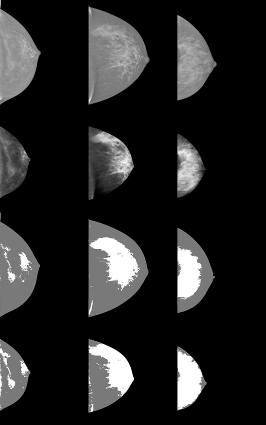
In the assessment of breast density from mammograms, the breast is usually considered as a two-component model consisting of adipose and fibroglandular (abbreviated as glandular hereafter) tissue to varying degrees. A user-assisted binary labeling technique is often used to estimate breast density . With this approach, image areas are labeled as radiographically dense tissue (glandular tissue) or as nondense (adipose) tissue. Breast density is then calculated as the ratio of the radiographically dense area to the total breast area (dense + nondense). We refer to this binary labeling technique as the standard user-assisted percentage of breast density (PD) measure (ie, the percent density measure).

Get Radiology Tree app to read full this article<

Materials and methods

Imaging System

Get Radiology Tree app to read full this article<

Study Population and Data Collection

Get Radiology Tree app to read full this article<

Calibration

Get Radiology Tree app to read full this article<

Percent Density

Get Radiology Tree app to read full this article<

Calibrated Percent Density

Get Radiology Tree app to read full this article<

A(x,y)=k(1.0−exp[−p(x,y)ts]), A

(

)

(

−

exp

[

−

(

)

]

)

where t s is the system compressed breast thickness readout quantity expressed in centimeters for each image, and k = 5000 is an arbitrary constant. Each calibrated image of the case-control dataset was transformed with Equation 1 producing the A(x,y) representation (case-control) dataset. Equation 1 is a variant of Beer’s law that can be used to define an idealized attenuated x-ray beam fractional measure [ie, A(x,y)/k]. The support for this relationship follows from the calibration methods outlined in the Appendix . This transform restricts the pixel values of A(x, y) within this range (0, k), and lends itself to a useful interpretation discussed below.

Get Radiology Tree app to read full this article<

PDc=dndn+an×100%, PD

100

where PD c indicates the PD-type measure was generated from calibrated data. The quantity d n + a n is the number of pixels within the eroded breast area. The other variant used the total breast area of the noneroded image in the denominator as the normalization.

Get Radiology Tree app to read full this article<

Analysis Methods

Get Radiology Tree app to read full this article<

Results

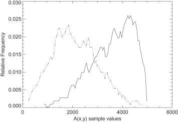
Breast Tissue Distributions

Get Radiology Tree app to read full this article<

Breast Density Measurement Comparisons

Get Radiology Tree app to read full this article<

Table 1

Patient Characteristics

Characteristic Case, n Case Mean (SD) or % Control, n Control Mean (SD) or % Age 106 58.91 (9.95) 106 58.71 (9.86) HRT Never 56 52.83% 61 57.55% 1–5 y 18 16.98% 15 14.15% 6–10 y 13 12.26% 14 13.21% 11–15 y 8 7.55% 7 6.60% >15 y 11 10.38% 9 8.49% BMI (kg/m 2 ) 106 26.86 (4.49) 106 25.51 (4.36)

This gives the number of observations ( n ) in the case and control groups, hormone replacement therapy (HRT) distribution by years of usage, and the mean body mass index (BMI), mean age, and associated standard deviation (SD).

Table 2

Percent Glandular and Percentage of Breast Density Associations

Measure: PG

Quartile OR (95% CI) Cases/controls Az (SE) Unadjusted 0.56 (0.02) 1 1.00 (ref.) 17/27 2 1.89 (0.81‒4.43) 30/26 3 2.01 (0.87‒4.63) 33/27 4 1.73 (0.69‒4.34) 26/26 BMI adjusted 0.62 (0.02) 1 1.00 (ref.) 17/27 2 1.96 (0.82‒4.72) 30/26 3 2.37 (0.99‒5.62) 33/27 4 2.43 (0.92‒6.49) 26/26

Measure: PD Unadjusted 0.61(0.02) 1 1.00 (ref.) 10/26 2 2.39 (0.96‒5.97) 26/27 3 3.78 (1.51‒9.43) 39/27 4 3.12 (1.23‒7.95) 31/26 BMI adjusted 0.68 (0.04) 1 1.00 (ref.) 10/26 2 2.88 (1.09‒7.57) 26/27 3 4.81 (1.82‒12.67) 39/27 4 5.09 (1.73‒15.02) 31/26

The percent glandular (PG) and percent density (PD) findings are presented in both unadjusted and adjusted for body mass index (BMI) quantities. The odds ratios (ORs) are shown by quartile with 95% confidence intervals (CIs). The number of case/control samples for each quartile is given in the third column. The area under the receiver operating characteristic curve (Az) and its standard error (SE) are also provided.

Table 3

Calibrated Percent Density Associations

Measure: PD c Total Area

Quartile OR (95% CI) Cases/controls Az (SE) Unadjusted 0.59 (0.02) 1 1.00 (ref.) 11/26 2 2.94 (1.17‒7.36) 32/27 3 3.01 (1.13‒8.02) 29/26 4 3.83 (1.39‒10.50) 34/27 BMI adjusted 0.65 (0.03) 1 1.00 (ref.) 11/26 2 3.44 (1.32‒8.99) 32/27 3 3.60 (1.29‒10.06) 29/26 4 5.62 (1.89‒16.76) 34/27

Measure: PD c eroded area Unadjusted 0.59 (0.02) 1 1.00 (ref.) 11/26 2 3.11 (1.24‒7.81) 32/27 3 3.14 (1.17‒8.39) 28/26 4 3.74 (1.40‒9.99) 35/27 BMI adjusted 0.65 (0.03) 1 1.00 (ref.) 11/26 2 3.67 (1.39‒9.63) 32/27 3 3.76 (1.34‒10.56) 28/26 4 5.46 (1.88‒15.80) 35/27

The calibrated percent density (PD c ) measure was derived by applying a static threshold to the transformed percent glandular (PG) representation images. The findings are presented with the total breast area normalization ( top ) and eroded area normalization ( bottom ). All findings are presented in unadjusted and adjusted for body mass index (BMI) quantities. The odds ratios (ORs) are presented by quartile with 95% confidence intervals (CIs). The number of case/control samples for each quartile is provided in the third column. The area under the receiver operating characteristic curve (Az) and its standard error (SE) are also provided.

Get Radiology Tree app to read full this article<

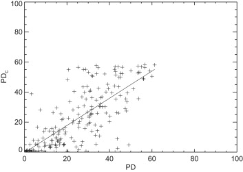
Table 4

Breast Density Measurement Distribution Summary

BD Measure Cases Mean (SD) Controls Mean (SD) PG 20.5 (18.4) 19.3 (14.1) PD 26.5 (15.6) 22.1 (17.4) PD c Total area 27.2 (19.1) 22.3 (19.9) PD c Eroded area 48.2 (33.9) 39.7 (35.4)

The three breast density (BD) distribution summaries are shown: percent glandular (PG), percent density (PD), and PD generated from the calibrated data (PD c ). The mean and standard deviation (SD) for each breast density measure are provided by case and control group.

Get Radiology Tree app to read full this article<

PG(x,y)≥−1tsln(1−Ack)×100. PG

(

)

≥

−

(

−

)

100

The threshold for the PG representation images is now dependent on t s (ie, image dependent) because the other terms on the right side of Equation 3 are constants.

Get Radiology Tree app to read full this article<

Discussion

Get Radiology Tree app to read full this article<

Acknowledgments

Get Radiology Tree app to read full this article<

Supplementary data

Get Radiology Tree app to read full this article<

Appendix

Get Radiology Tree app to read full this article<

References

1. Boyd N.F., Rommens J.M., Vogt K., et. al.: Mammographic breast density as an intermediate phenotype for breast cancer. Lancet Oncol 2005; 6: pp. 798-808.
2. McCormack V.A., dos Santos Silva I.: Breast density and parenchymal patterns as markers of breast cancer risk: a meta-analysis. Cancer Epidemiol Biomarkers Prev 2006; 15: pp. 1159-1169.
3. Boyd N.F., Guo H., Martin L.J., et. al.: Mammographic density and the risk and detection of breast cancer. N Engl J Med 2007; 356: pp. 227-236.
4. Harvey J.A., Bovbjerg V.E.: Quantitative assessment of mammographic breast density: relationship with breast cancer risk. Radiology 2004; 230: pp. 29-41.
5. Yaffe M.J.: Mammographic density. Measurement of mammographic density. Breast Cancer Res 2008; 10: pp. 209.
6. Byng J.W., Boyd N.F., Fishell E., et. al.: The quantitative analysis of mammographic densities. Phys Med Biol 1994; 39: pp. 1629-1638.
7. Boyd N.F., Byng J.W., Jong R.A., et. al.: Quantitative classification of mammographic densities and breast cancer risk: results from the Canadian National Breast Screening Study. J Natl Cancer Inst 1995; 87: pp. 670-675.
8. Boyd N.F., Lockwood G.A., Byng J.W., et. al.: Mammographic densities and breast cancer risk. Cancer Epidemiol Biomarkers Prev 1998; 7: pp. 1133-1144.
9. Highnam R., Brady M.: Mammographic Image Analysis.1999.Kluwer Academic PublishersBoston, MA
10. Kaufhold J., Thomas J.A., Eberhard J.W., et. al.: A calibration approach to glandular tissue composition estimation in digital mammography. Med Phys 2002; 29: pp. 1867-1880.
11. Pawluczyk O., Augustine B.J., Yaffe M.J., et. al.: A volumetric method for estimation of breast density on digitized screen-film mammograms. Med Phys 2003; 30: pp. 352-364.
12. Shepherd J.A., Herve L., Landau J., et. al.: Novel use of single X-ray absorptiometry for measuring breast density. Technol Cancer Res Treat 2005; 4: pp. 173-182.
13. Heine J.J., Behera M.: Effective x-ray attenuation measurements with full field digital mammography. Med Phys 2006; 33: pp. 4350-4366.
14. van Engeland S., Snoeren P.R., Huisman H., et. al.: Volumetric breast density estimation from full-field digital mammograms. IEEE Trans Med Imaging 2006; 25: pp. 273-282.
15. Highnam R., Pan X., Warren R., et. al.: Breast composition measurements using retrospective standard mammogram form (SMF). Phys Med Biol 2006; 51: pp. 2695-2713.
16. Heine J.J., Thomas J.A.: Effective x-ray attenuation coefficient measurements from two full field digital mammography systems for data calibration applications. Biomed Eng Online 2008; 7: pp. 13.
17. Malkov S., Wang J., Kerlikowske K., et. al.: Single x-ray absorptiometry method for the quantitative mammographic measure of fibroglandular tissue volume. Med Phys 2009; 36: pp. 5525-5536.
18. Ding J., Warren R., Warsi I., et. al.: Evaluating the effectiveness of using standard mammogram form to predict breast cancer risk: case-control study. Cancer Epidemiol Biomarkers Prev 2008; 17: pp. 1074-1081.
19. Boyd N., Martin L., Gunasekara A., et. al.: Mammographic density and breast cancer risk: evaluation of a novel method of measuring breast tissue volumes. Cancer Epidemiol Biomarkers Prev 2009; 18: pp. 1754-1762.
20. Heine J.J., Cao K., Beam C.: Cumulative sum quality control for calibrated breast density measurements. Med Phys 2009; 36: pp. 5380-5390.
21. Heine J.J., Cao K., Thomas J.A.: Effective radiation attenuation calibration for breast density: compression thickness influences and correction. Biomed Eng Online 2010; 9: pp. 73.
22. Mahesh M.: AAPM/RSNA physics tutorial for residents: digital mammography: an overview. Radiographics 2004; 24: pp. 1747-1760.
23. Vedantham S., Karellas A., Suryanarayanan S., et. al.: Full breast digital mammography with an amorphous silicon-based flat panel detector: physical characteristics of a clinical prototype. Med Phys 2000; 27: pp. 558-567.
24. Heine J.J., Carston M.J., Scott C.G., et. al.: An automated approach for estimation of breast density. Cancer Epidemiol Biomarkers Prev 2008; 17: pp. 3090-3097.
25. Jeffreys M., Warren R., Highnam R., et. al.: Initial experiences of using an automated volumetric measure of breast density: the standard mammogram form. Br J Radiol 2006; 79: pp. 378-382.
26. Parzen E.: On estimation of a probability density function and mode. Ann Mathemat Stat 1962; 33: pp. 1065-1076.
27. Cacoullos T.: Estimation of a multivariate density. Ann Inst Statist Math 1966; 18: pp. 179-189.
28. Specht D.F.: A general regression neural network. IEEE Transactions on Neural Networks 1991; 2: pp. 568-576.

A Quantitative Description of the Percentage of Breast Density Measurement Using Full-field Digital Mammography

Rationale and Objectives

Materials and Methods

Results

Conclusions

Materials and methods

Imaging System

Study Population and Data Collection

Calibration

Percent Density

Calibrated Percent Density

Analysis Methods

Results

Breast Tissue Distributions

Breast Density Measurement Comparisons

Discussion

Acknowledgments

Supplementary data

References

Further Reading

A Dedicated General Competencies Curriculum for Radiology Residents

An Anthropomorphic Breast Model for Breast Imaging Simulation and Optimization

Beginning Medicare