
Rationale and Objectives
Estimation of regional lung function parameters from hyperpolarized gas magnetic resonance images can be very sensitive to presence of noise. Clustering pixels and averaging over the resulting groups is an effective method for reducing the effects of noise in these images, commonly performed by grouping proximal pixels together, thus creating large groups called “bins.” This method has several drawbacks, primarily that it can group dissimilar pixels together, and it degrades spatial resolution. This study presents an improved approach to simplifying data via principal component analysis (PCA) when noise level prohibits a pixel-by-pixel treatment of data, by clustering them based on similarity to one another rather than spatial proximity. The application to this technique is demonstrated in measurements of regional lung oxygen tension using hyperpolarized 3 He magnetic resonance imaging (MRI).
Materials and Methods
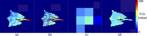
A synthetic dataset was generated from an experimental set of oxygen tension measurements by treating the experimentally derived parameters as “true” values, and then solving backwards to generate “noiseless” images. Artificial noise was added to the synthetic data, and both traditional binning and PCA-based clustering were performed. For both methods, the root-mean-square (RMS) error between each pixel’s “estimated” and “true” parameters was computed and the resulting effects were compared.
Results
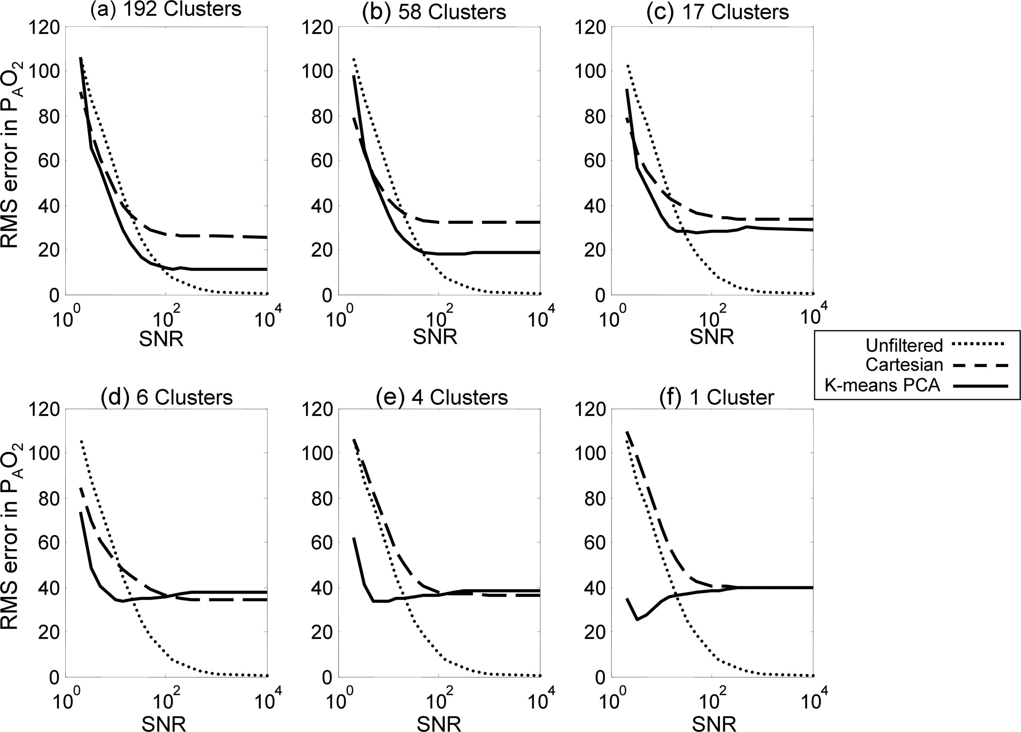
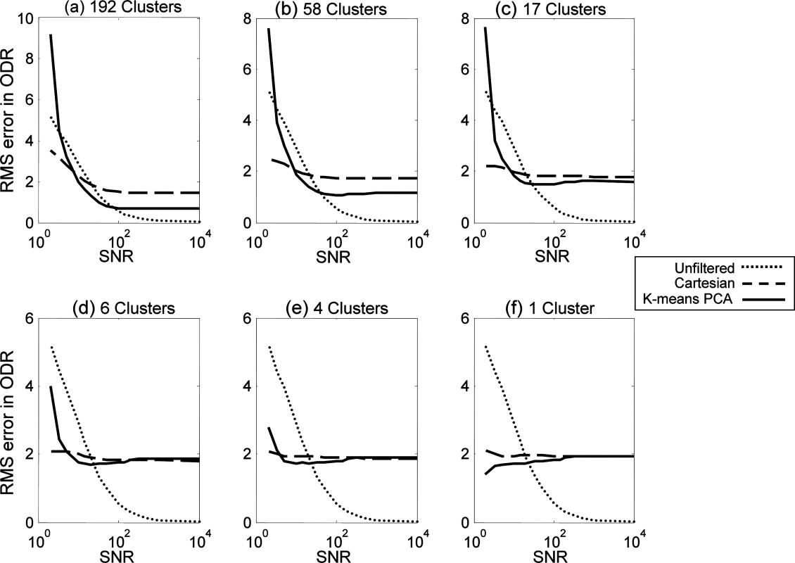
At high signal-to-noise ratios (SNRs), clustering did not enhance accuracy. Clustering did, however, improve parameter estimations for moderate SNR values (below 100). For SNR values between 100 and 20, the PCA-based K-means clustering analysis yielded greater accuracy than Cartesian binning. In extreme cases (SNR < 5), Cartesian binning can be more accurate.
Conclusions
The reliability of parameters estimation in imaging-based regional functional measurements can be improved in the presence of noise by utilizing principal component analysis-based clustering without sacrificing spatial resolution compared to Cartesian binning. Results suggest that this approach has a great potential for robust grouping of pixels in hyperpolarized 3 He MRI maps of lung oxygen tension.
Pulmonary disorders such as emphysema, asthma, and acute respiratory distress syndrome are among the most common illnesses in the world; asthma alone is estimated to afflict 150 million people globally and costs the Untied States over $6 billion each year ( ). Emphysema may impact over 3% of the United States population, which is more than 9 million people ( ). Because the lung is a large and heterogeneous organ, these conditions can be difficult to diagnose clinically. It is thus important to develop sensitive radiologic techniques for regional measurement of lung function to assist physicians in diagnosing such diseases.
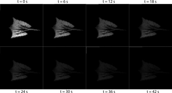
Functional lung imaging using hyperpolarized gas magnetic resonance imaging (HP gas MRI) allows various pulmonary parameters to be assessed regionally (3). This method is safe and does not deliver ionizing radiation to patients. Patients inhale hyperpolarized helium-3 ( 3 He) or xenon-129 ( 129 Xe), and images of the airspaces are subsequently acquired. Signal intensity in each region of the lungs is directly related to the degree of polarization of the gas and the amount of gas that is present in that region. The images can be postprocessed to reveal physiologic information. HP gas MRI allows researchers to rigorously assess a wide range of pulmonary parameters, such as regional ventilation ( ), the regional alveolar partial pressure of oxygen (P A O 2 ) ( ), and the apparent diffusion coefficient (ADC) of gasses, which is linked to the size of the alveoli and structure of small airway ( ), turning them into powerful tools for diagnosing and studying lung diseases.
Get Radiology Tree app to read full this article<
Get Radiology Tree app to read full this article<
Get Radiology Tree app to read full this article<
Get Radiology Tree app to read full this article<
Get Radiology Tree app to read full this article<
Theory
Measurement of Regional Oxygen Tension
Get Radiology Tree app to read full this article<
ΓO2=PAO2ξ, Γ
O
2
=
P
A
O
2
ξ
,
where ξ = 2.6 bar · s at body temperature. The decay rate, however, is different for each region, and is a function of local P A O 2 and ODR. Theoretically, this relation is given by the following equation for the n -th image in the sequence ( ):
S(n)=S(0)⋅exp[M⋅n⋅ln(cos(α))−1ξ(PAO2⋅t(n)−12ODR⋅t2(n))], S
(
n
)
=
S
(
0
)
·
e
xp
[
M
·
n
·
ln
(
cos
(
α
)
)
−
1
ξ
(
P
A
O
2
·
t
(
n
)
−
1
2
ODR
·
t
2
(
n
)
)
]
,
where S (0) indicates the original signal intensity in each region. In general the interscan time delay t ( n ) can be an arbitrary function of the image number n . In the case of equally spaced images, t ( n ) = τ · n , where τ is the time interval between each pair of images. The form of Equation 2 follows from the common approximation that uptake of oxygen into the blood stream can be expressed as a linear function:
PAO2(t)=PAO2(0)−ODR⋅t P
A
O
2
(
t
)
=
P
A
O
2
(
0
)
−
O
DR
·
t
where P A O 2 (0) denotes oxygen partial pressure at the beginning of the breathhold ( t = 0). If two images are obtained with no—or negligible with respect to Γ O2 —interscan time delay in each slice at the beginning of the image series, they can be used to fairly accurately calculate the flip angle in each region of the lung by analyzing the signal decay induced by RF pulse. Subsequent images are obtained at longer time intervals, and are used to calculate signal decay caused by oxygen. The time evolution of P A O 2 ( t ) and ODR( t ) values at acquisition times can therefore be obtained in this manner from a single series of images acquired during one single breathhold ( ).
Get Radiology Tree app to read full this article<
Formation of the Data Space
Get Radiology Tree app to read full this article<
Principal Component Analysis
Get Radiology Tree app to read full this article<
Get Radiology Tree app to read full this article<
Get Radiology Tree app to read full this article<
B=X−u⋅h B
=
X
−
u
⋅
h
where h is a 1 × N vector of all ones. Next, the covariance matrix C is computed and its unit eigenvectors V__n (1 ≤ n ≤ A) are determined, as are their corresponding eigenvalues l__n . C is given by:
C=1A−1B⋅B*, C
=
1
A
−
1
B
·
B
*
,
where * represents the conjugate transpose operation. The eigenvectors are sorted in decreasing order of eigenvalues l . By theorem, these unit eigenvectors are orthogonal to one another, and they define a space identical to the data space ( ). The eigenvector corresponding to the highest eigenvalue is the first principal component, and the following eigenvectors represent the remaining principal components in decreasing order of eigenvalues. Also, the eigenvalue of the n -th principal component tells us what proportion P of the variation in the data it describes, as given by the identity:
P=λnλ1+⋅⋅⋅+λN. P
=
λ
n
λ
1
+
⋅
⋅
⋅
+
λ
N
.
We assume that projecting all our data points into the two-dimensional space defined by the first two principal components effectively eliminates variation in the data due to insignificant variables, although this property cannot be universally assumed. The desired result is a lower dimension data space in which noise effects has been reduced. Clustering points in this reduced data space can theoretically allow parameters estimations to be performed with less uncertainty in presence of noise.
Get Radiology Tree app to read full this article<
Data Clustering—Cartesian Binning and K-means
Get Radiology Tree app to read full this article<
Get Radiology Tree app to read full this article<
v=∑ki=1∑xj∈Si∣∣xj−μi|2, v
=
∑
i
=
1
k
∑
x
j
∈
S
i
|
x
j
−
μ
i
|
2
,
where each S__i is a cluster with the centroid μ__i . Objects are moved between clusters until v is minimized. The theoretical result is a set of clusters that are as compact and separated as possible.
Get Radiology Tree app to read full this article<
Get Radiology Tree app to read full this article<
Materials and methods
Helium-3 Polarization
Get Radiology Tree app to read full this article<
Animal Preparation
Get Radiology Tree app to read full this article<
Oxygen Tension Measurement Experiment
Get Radiology Tree app to read full this article<
Imaging Protocol
Get Radiology Tree app to read full this article<
Data Analysis
Get Radiology Tree app to read full this article<
Synthetic Data
Get Radiology Tree app to read full this article<
SNR=1NS2−N2,−−−−−−−−√ S
N
R
=
1
N
S
2
−
N
2
,
where S is the signal intensity of the pixel, and N is the bias-corrected noise level in the image ( ):
N=2π⋅Nˆ.−−−−−−√ N
=
2
π
·
N
.
The unbalanced noise, Nˆ N
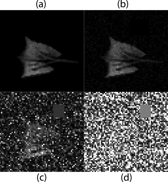
, is estimated by averaging the intensity of a group of pixels in an area of the image in which no MR signal is present, away from the actual lung tissue. Pixels not exceeding an SNR = 3 in the first image of the series were excluded in the synthetic dataset. The synthetic data was only generated for a single slice near the middle of the lung that contained the trachea.
Get Radiology Tree app to read full this article<
Principal Component Analysis
Get Radiology Tree app to read full this article<
Data Clustering
Get Radiology Tree app to read full this article<
Noise Simulations
Get Radiology Tree app to read full this article<
Comparison of Clustering Techniques
Get Radiology Tree app to read full this article<
Results
Experimental Data and Synthetic Images
Get Radiology Tree app to read full this article<
Get Radiology Tree app to read full this article<
Principal Component Analysis
Get Radiology Tree app to read full this article<
Get Radiology Tree app to read full this article<
Oxygen Parameter Estimation in the Synthetic Dataset
Get Radiology Tree app to read full this article<
Get Radiology Tree app to read full this article<
Get Radiology Tree app to read full this article<
Get Radiology Tree app to read full this article<
Discussion
Principal Component Analysis
Get Radiology Tree app to read full this article<
Oxygen Parameter Estimation
Get Radiology Tree app to read full this article<
Number of Clusters
Get Radiology Tree app to read full this article<
Get Radiology Tree app to read full this article<
Potential Clinical Applications
Get Radiology Tree app to read full this article<
Study Limitations
Get Radiology Tree app to read full this article<
Get Radiology Tree app to read full this article<
Get Radiology Tree app to read full this article<
Get Radiology Tree app to read full this article<
Conclusions
Get Radiology Tree app to read full this article<
Get Radiology Tree app to read full this article<
References
1. Cookson W.: The alliance of genes and environment in asthma and allergy. Nature 1999; 402: pp. B5-B11.
2. Boutin-Forzano S., Moreau D., Kalaboka S., et. al.: Reported prevalence and co-morbidity of asthma, chronic bronchitis and emphysema: a pan-European estimation. Int J Tuberc Lung Dis 2007; 11: pp. 695-702.
3. Ishii M., Fischer M.C., Emami K., et. al.: Hyperpolarized 3 He MR imaging of pulmonary function. Radiol Clin North Am 2005; 43: pp. 235-246.
4. Deninger A.J., Månsson S., Petersson J.S., et. al.: Quantitative measurement of regional lung ventilation using 3 He MRI. Magn Reson Med 2002; 48: pp. 223-232.
5. Deninger A.J., Eberle B., Ebert M., et. al.: Quantification of regional intrapulmonary oxygen partial pressure evolution during apnea by (3)He MRI. J Magn Reson 1999; 141: pp. 207-216.
6. Fain S.B., Panth S.R., Evans M.D., et. al.: Early emphysematous changes in asymptomatic smokers: detection with 3 He MR imaging. Radiology 2006; 239: pp. 875-883.
7. Fischer M.C., Spector Z.Z., Ishii M., et. al.: Single-acquisition sequence for the measurement of oxygen partial pressure by hyperpolarized gas MRI. Magn Reson Med 2004; 52: pp. 766-773.
8. Fischer M.C., Kadlecek S., Yu J., et. al.: Measurements of regional alveolar oxygen pressure using hyperpolarized 3 He MRI. Acad Radiol 2005; 12: pp. 1430-1439.
9. Shiga M., Takigawa I., Mamitsuka H.: Annotating gene function by combining expression data with a modular gene network. Bioinformatics 2007; 23: pp. i468-i478.
10. Banada P.P., Guo S., Bayraktar B., et. al.: Optical forward-scattering for detection of Listeria monocytogenes and other Listeria species. Biosense Bioelectron 2007; 22: pp. 1664-1671.
11. Wang Z., Wang J., Calhoun V., et. al.: Strategies for reducing large fMRI data sets for independent component analysis. Magn Reson Imaging 2006; 24: pp. 591-596.
12. Goutte C., Hansen L.K., Liptrot M.G., et. al.: Feature-space clustering for fMRI meta-analysis. Hum Brain Mapp 2001; 13: pp. 165-183.
13. Goutte C., Toft P., Rostrup E., et. al.: On clustering fMRI time series. Neuroimage 1999; 9: pp. 298-310.
14. Kimura Y., Hsu H., Toyama H., et. al.: Improved signal-to-noise ratio in parametric images by cluster analysis. Neuroimage 1999; 9: pp. 554-561.
15. Kimura Y., Senda M., Alpert N.M.: Fast formation of statistically reliable FDG parametric images based on clustering and principal components. Phys Med Biol 2002; 47: pp. 455-468.
16. Layfield D., Venegas J.G.: Enhanced parameter estimation from noisy PET data: Part I–methodology. Acad Radiol 2005; 12: pp. 1440-1447.
17. Yu J., Ishii M., Kadlecek S., et. al.: Multiple regression method for pulmonary apparent diffusion coefficient measurement by hyperpolarized 3 He MRI. J Magn Reson Imaging 2007; 25: pp. 982-991.
18. MATLAB Statistics Toolbox, User’s Guide, 5th Ed. Natick, MA: MathWorks, 2004.
19. Lay D.: Linear Algebra and its Applications.2003.Addison WesleyNew York, NY
20. Ding C., Xe H.: K-means clustering via principal component analysis. Proc Int’l Conf Machine Learning 2004; pp. 225-232.
21. Gudbjartsson H., Patz S.: The Rician distribution of noisy MRI data. Magn Reson Med 1995; 34: pp. 910-914.
22. Venegas J.G., Winkler T., Musch G., et. al.: Self-Organized Patchiness in Asthma as a Prelude to Catastrophic Shifts. Nature 2005; 434: pp. 777-782.
23. Roberts D.A., Rizi R.R., Lipson D.A., et. al.: Detection and localization of pulmonary air leaks using laser-polarized (3)He MRI. Magn Reson Med 2000; 44: pp. 379-382.