
Rationale and Objectives
We propose a novel segmentation-based interpolation method to reduce the metal artifacts caused by surgical aneurysm clips.
Materials and Methods
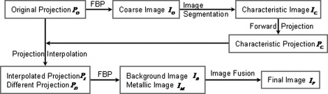
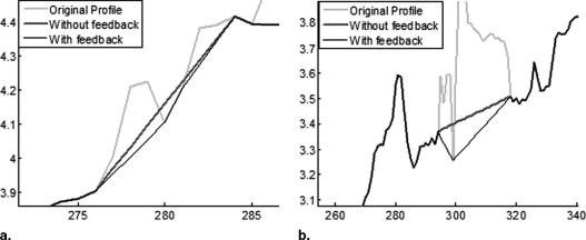
Our method consists of five steps: coarse image reconstruction, metallic object segmentation, forward-projection, projection interpolation, and final image reconstruction. The major innovations are 2-fold. First, a state-of-the-art mean-shift technique in the computer vision field is used to improve the accuracy of the metallic object segmentation. Second, a feedback strategy is developed in the interpolation step to adjust the interpolated value based on the prior knowledge that the interpolated values should not be larger than the original ones. Physical phantom and real patient datasets are studied to evaluate the efficacy of our method.
Results
Compared to the state-of-the-art segmentation-based method designed previously, our method reduces the metal artifacts by 20–40% in terms of the standard deviation and provides more information for the assessment of soft tissues and osseous structures surrounding the surgical clips.
Conclusion
Mean shift technique and feedback strategy can help to improve the image quality in terms of reducing metal artifacts.
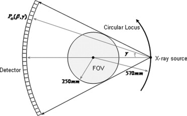
In x-ray computed tomography (CT), the attenuation coefficient of high-density objects, such as surgical clips, metal prostheses, or dental amalgams, is much higher than that of soft tissues and osseous structures. Because the x-ray beam is highly attenuated by metals, an insufficient number of photons reach the detector, producing corrupted projection data. Consequently, images reconstructed by the traditional filtered back-projection (FBP) method are marred by starburst artifacts, often referred to as metal artifacts. These artifacts significantly degrade CT image quality and limit the usefulness of CT for many clinical applications because tissues in the plane of the metal appliance are severely obscured. Hence, there is an important need for methods that reduce metal artifacts.
The effects of metallic objects on x-ray scanning are 2-fold: beam hardening, due to the poly-energetic x-ray spectrum, and a poor signal-to-noise ratio from photon starvation. To suppress the metal artifacts, iterative reconstruction methods have been successfully applied that avoid the corrupted data. For example, Wang et al. used the maximum expectation maximization (EM) formula and algebraic reconstruction technique (ART) to iteratively deblur metallic artifact ( ). A key step in their algorithm is the introduction of a projection mask and the computation of a 3D spatially varying relaxation factor that allows compensation for beam divergence and data incompleteness. However, this approach is computationally expensive and not practical for clinical imaging. Conventional FBP methods ( ) are computationally efficient but produce image artifacts when complete and precise projection data are unavailable. Different linear and polynomial interpolation techniques have been developed for estimating the “missing” projection data ( ). The major task of this method is to identify the corrupted segments in the sinogram and interpolate these data from noncorrupted neighbor projections. Because the first step of all the above methods requires segmenting of the metal parts from a coarse image reconstructed by FBP, segmentation is a key technique for metal artifact reduction.
Get Radiology Tree app to read full this article<
Get Radiology Tree app to read full this article<
Methods
Algorithm Description
Get Radiology Tree app to read full this article<
Get Radiology Tree app to read full this article<
Step 1: Coarse image reconstruction
Get Radiology Tree app to read full this article<
Step 2: Metallic object segmentation
Get Radiology Tree app to read full this article<
IC(m,n)={10ifIO(m,n)belongs to metallic objectsotherwise, I
C
(
m
,
n
)
=
{
1
if
I
O
(
m
,
n
)
belongs to metallic objects
0
otherwise
,
where the subscript “ C ” denotes a characteristic function. I C functions as an index for the metallic objects in the specified ROI. In the next subsection, we describe this procedure in detail.
Get Radiology Tree app to read full this article<
Step 3: Forward-projection
Get Radiology Tree app to read full this article<
PC(βi,γj)={10PM(βi,γj)>0otherwise. P
C
(
β
i
,
γ
j
)
=
{
1
P
M
(
β
i
,
γ
j
)
0
0
otherwise
.
Get Radiology Tree app to read full this article<
Get Radiology Tree app to read full this article<
Step 4: Projection interpolation
Get Radiology Tree app to read full this article<
PD(βi,γj)=PO(βi,γj)−PI(βi,γj). P
D
(
β
i
,
γ
j
)
=
P
O
(
β
i
,
γ
j
)
−
P
I
(
β
i
,
γ
j
)
.
Get Radiology Tree app to read full this article<
Get Radiology Tree app to read full this article<
Step 5: Final image reconstruction
Get Radiology Tree app to read full this article<
IF(m,n)=IB(m,n)+η×I∗C(m,n)×IM(m,n), I
F
(
m
,
n
)
=
I
B
(
m
,
n
)
+
η
×
I
C
*
(
m
,
n
)
×
I
M
(
m
,
n
)
,
where η is the scale factor, ranging from 0.05 to 0.5, and I C * functions as a mask to protect the background image from corruption by the metallic artifacts. To smooth the edge and preserve the structure of the metallic objects, I C * is defined as the 2D convolution of the characteristic image I C and a normalized Gaussian kernel.
Get Radiology Tree app to read full this article<
Metallic Object Segmentation
Get Radiology Tree app to read full this article<
Get Radiology Tree app to read full this article<
MS(x)=∑Kk=1G(xk−x)W(xk)xk∑Kk=1G(xk−x)W(xk). M
S
(
x
)
=
∑
k
=
1
K
G
(
x
k
−
x
)
W
(
x
k
)
x
k
∑
k
=
1
K
G
(
x
k
−
x
)
W
(
x
k
)
.
Get Radiology Tree app to read full this article<
Get Radiology Tree app to read full this article<
Get Radiology Tree app to read full this article<
G(x)=Ch2shrg(∥xs/hs∥2)g(∥xr/hr∥2), G
(
x
)
=
C
h
s
2
h
r
g
(
‖
x
s
/
h
s
‖
2
)
g
(
‖
x
r
/
h
r
‖
2
)
,
with the common profile
g(s)={10|s|<1otherwise. g
(
s
)
=
{
1
|
s
|
<
1
0
otherwise
.
Get Radiology Tree app to read full this article<
Get Radiology Tree app to read full this article<
IG(m,n)=|∇IO(m,n)|=(∂IO(m,n)∂m)2+(∂IO(m,n)∂n)2−−−−−−−−−−−−−−−−−−−−√. I
G
(
m
,
n
)
=
|
∇
I
O
(
m
,
n
)
|
=
(
∂
I
O
(
m
,
n
)
∂
m
)
2
+
(
∂
I
O
(
m
,
n
)
∂
n
)
2
.
Get Radiology Tree app to read full this article<
Get Radiology Tree app to read full this article<
W(m,n)=1−λIG(m,n)/max(IG), W
(
m
,
n
)
=
1
−
λ
I
G
(
m
,
n
)
/
max
(
I
G
)
,
where max( I G ) is the maximum of the gradient image I G and 0 ≤ γ < 1 is a scale factor. As a result, all the necessary components have been determined for the mean shift technique.
Get Radiology Tree app to read full this article<
Get Radiology Tree app to read full this article<
Get Radiology Tree app to read full this article<
Get Radiology Tree app to read full this article<
Get Radiology Tree app to read full this article<
Get Radiology Tree app to read full this article<
Feedback-Based Interpolation Strategy
Get Radiology Tree app to read full this article<
Get Radiology Tree app to read full this article<
Get Radiology Tree app to read full this article<
Get Radiology Tree app to read full this article<
Get Radiology Tree app to read full this article<
Results
Algorithm Implementation
Get Radiology Tree app to read full this article<
Table 1
Parameter Selection for our Phantom and Patient Datasets
Phantom Dataset Patient Dataset Pixel size (mm 2 ) 0.135 × 0.135 0.164 × 0.164 Spatial domain bandwidth h s (mm) 0.33 0.82 Range domain bandwidth h r (HU) 1000 1500 Coefficient for weighting function λ 0.5 0.5 Threshold for metallic segmentation (HU) 1500 3500 Scale factor for final reconstruction η 0.15 0.15
Get Radiology Tree app to read full this article<
Get Radiology Tree app to read full this article<
Clip Phantom Experiment
Get Radiology Tree app to read full this article<
D=∑m,n(IF(m,n)−T)2×DC(m,n)∑m,nDC(m,n)−−−−−−−−−−−−−−−−−−−√ D
=
∑
m
,
n
(
I
F
(
m
,
n
)
−
T
)
2
×
D
C
(
m
,
n
)
∑
m
,
n
D
C
(
m
,
n
)
![Figure 5, Representative images of the clip phantom reconstructed using different methods. The left column images were directly reconstructed from the fan-beam sinogram without any correction. The middle column images were corrected using the conventional segmentation-based interpolation method. The right column images were corrected using our proposed method. The middle row images are the local magnification of the top row. The bottom row images are the characteristic functions for quantitative measurement of the middle row images. The significant differences between (e) and (f) are indicated by arrows. The display windows are [−100,300] HU.](https://storage.googleapis.com/dl.dentistrykey.com/clinical/ASegmentationBasedMethodforMetalArtifactReduction/4_1s20S1076633207000025.jpg)
Get Radiology Tree app to read full this article<
Get Radiology Tree app to read full this article<
Table 2
Standard Deviations Associated with Different Correction Methods
Without Correction Wei et al. Method Our Method Clip phantom 681.80 181.12 142.66 Patent head 1759.91 330.27 186.09
Get Radiology Tree app to read full this article<
Patient Study
Get Radiology Tree app to read full this article<
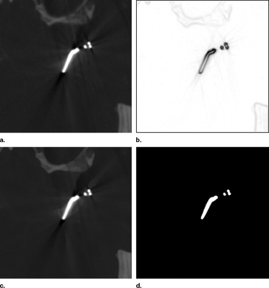
![Figure 6, Representative images of the patient head reconstructed using different methods. The left column image were directly reconstructed from the fan-beam sinogram without any correction. The middle column images were corrected using the conventional segmentation-based interpolation method. The right column images were corrected using our proposed method. The middle row images are the local magnification of the top row images. The bottom row images are the characteristic functions for quantitative measurement of the middle row images. The significant differences between (e) and (f) are indicated by circles. The display windows are [−100,300] HU.](https://storage.googleapis.com/dl.dentistrykey.com/clinical/ASegmentationBasedMethodforMetalArtifactReduction/5_1s20S1076633207000025.jpg)
Get Radiology Tree app to read full this article<
Discussion
Get Radiology Tree app to read full this article<
Get Radiology Tree app to read full this article<
Conclusion
Get Radiology Tree app to read full this article<
Get Radiology Tree app to read full this article<
References
1. Wang G., Snyder D.L., Osullivan J.A., Vannier M.W.: Iterative deblurring for CT metal artifact reduction. IEEE Trans Med Imaging 1996; 15: pp. 657-664.
2. Wang G., Vannier M.W., Cheng P.C.: Iterative X-ray cone-beam tomography for metal artifact reduction and local region reconstruction. Microsc Microanaly 1999; 5: pp. 58-65.
3. Kak A.C., Slaney M.: 1988.IEEE PressNew York
4. Mahnken A.H., Raupach R., Wildberger J.E., et. al.: A new algorithm for metal artifact reduction in computed tomography - In vitro and in vivo evaluation after total hip replacement. Investigative Radiology 2003; 38: pp. 769-775.
5. Kalender W.A., Hebel R., Ebersberger J.: Reduction of CT artifacts caused by metallic implants. Radiology 1987; 164: pp. 576-577.
6. Watzke O., Kalender W.A.: A pragmatic approach to metal artifact reduction in CT: merging of metal artifact reduced images. Eur Radiol 2004; 14: pp. 849-856.
7. Kudo H., Saito T.: Sinogram recovery with the method of convex projections for limited-data reconstruction in computed-tomography. J Optic Soc Am A Optics Image Sci Vision 1991; 8: pp. 1148-1160.
8. Zhao S.Y., Bae K.T., Whiting B., Wang G.: A wavelet method for metal artifact reduction with multiple metallic objects in the field of view. J X-ray Sci Technol 2002; 10: pp. 67-76.
9. Zhao S.Y., Robertson D.G., Bae K.T., Whiting B., Wang G.: X-ray CT metal artifact reduction using wavelets: An application for imaging total hip prostheses. IEEE Trans Med Imaging 2000; 19: pp. 1238-1247.
10. Wei J.K., Chen L.G., Sandison G.A., Liang Y., Xu L.X.: X-ray CT high-density artefact suppression in the presence of bones. Phys Med Biol 2004; 49: pp. 5407-5418.
11. Yazdi M., Gingras L., Beaulieu L.: An adaptive approach to metal artifact reduction in helical computed tomography for radiation therapy treatment planning: Experimental and clinical studies. Int J Radiat Oncol Biol Phys 2005; 62: pp. 1224-1231.
12. Bal M., Spies L.: Metal artifact reduction in CT using tissue-class modeling and adaptive prefiltering. Med Phys 2006; 33: pp. 2852-2859.
13. Cheng Y.Z.: Mean shift, mode seeking, and clustering. IEEE Trans Pattern Anal Machine Intellig 1995; 17: pp. 790-799.
14. Comaniciu D., Meer P.: Mean shift: A robust approach toward feature space analysis. IEEE Trans Pattern Anal Machine Intellig 2002; 24: pp. 603-619.
15. Noo F., Defrise M., Clackdoyle R.: Single-slice rebinning method for helical cone-beam CT. Phys Med Biol 1999; 44: pp. 561-570.
16. Chen L.G., Liang Y., Sandison G.A., Rydbery J.: Novel method for reducing high-attenuation object artifacts in CT reconstructions. Proc SPIE 2002; 4684: pp. 841-850.
17. Fukunaga K., Hostetler L.D.: The estimation of the gradient of a density function, with applications in pattern recognition. EEE Trans Infor Theory 1975; 21: pp. 32-40.
18. Comaniciu D., Ramesh V., Meer P.: The variable bandwidth mean shift and data-driven scale selection.8th IEEE International Conference on Computer Vision.2002.pp. 438-445.