
Rationale and Objectives
Metachromatic leukodystrophy is a lysosomal storage disorder leading to progressive demyelination of brain white matter. This is sensitively detected using magnetic resonance imaging. The volume of demyelination, the “demyelination load,” could serve as a useful parameter for assessing both the natural course of the disease and treatment effects. The aim of this study was to develop and validate a semiautomated approach for determining the demyelination load to achieve reliable and time-efficient segmentation results.
Materials and Methods
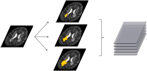
The demyelination load was determined in 77 magnetic resonance imaging data sets from 35 patients both manually and semiautomatically. For manual segmentation, regarded as the gold standard, the software ITK-Snap was used. For semiautomatic segmentation, a new algorithm called Clusterize was developed and implemented in MATLAB, consisting of automatic iterative region growing followed by the interactive selection of clusters. Results were compared in terms of the obtained volumes, spatial overlap, and time taken to conduct the segmentation.
Results
Performance of the semiautomatic algorithm was excellent, with the volumes generated by the new algorithm showing good agreement with the ones generated by the gold standard (93.4 ± 45.5 vs 96.1 ± 49.0 mL, P = NS) with high spatial overlap (Dice’s similarity coefficient = 0.7861 ± 0.0697). The semiautomatic algorithm was significantly faster than the gold standard (8.2 vs 27.0 min, P < .001). Intrarater and interrater reliability determined high reproducibility of the method.
Conclusion
The demyelination load in metachromatic leukodystrophy can be determined in a time-efficient manner using a semiautomatic algorithm, showing high agreement with the current gold standard.
Metachromatic leukodystrophy (MLD) is a rare inherited lysosomal storage disorder leading to the degradation of the myelin sheath in both the central and peripheral nervous system . Three forms are distinguished: a late infantile (onset before 3 years of age), a juvenile (16 years), and an adult form. Patients develop progressive neurologic symptoms with different rates of disease progression and different initial manifestations . Currently, no curative treatment is available, though promising new therapeutic approaches are under investigation .
The imaging hallmark of this disease is a rapidly progressive leukodystrophy, which can be detected sensitively using magnetic resonance (MR) imaging. Demyelinated white matter (WM) presents as hyperintensities on T2-weighted images. Only recently, Eichler et al developed a score for visually assessing these hyperintensities. This score ranges from 0 to 34 points and has been applied to describe the natural course of the disorder in children . Here, a rater scores a number of predefined brain regions as “normal” (healthy), “faint” (1 point), or “dense hyperintensity” (2 points). Although this allows the assessment of global disease progression in a structured way, it would be beneficial to have a more sensitive and quantitative measure of the affected tissue . This is particularly important when evaluating new therapeutic approaches, for which an objective validation of putative treatment-induced changes is of high relevance.
Get Radiology Tree app to read full this article<
Get Radiology Tree app to read full this article<
Materials and methods
MR Imaging Data
Get Radiology Tree app to read full this article<
Get Radiology Tree app to read full this article<
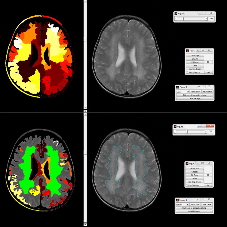
Manual Segmentation
Get Radiology Tree app to read full this article<
Get Radiology Tree app to read full this article<
Get Radiology Tree app to read full this article<
Get Radiology Tree app to read full this article<
Get Radiology Tree app to read full this article<
Semiautomatic Segmentation
Get Radiology Tree app to read full this article<
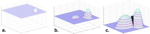
Automated preprocessing
Get Radiology Tree app to read full this article<
Get Radiology Tree app to read full this article<
Get Radiology Tree app to read full this article<
Get Radiology Tree app to read full this article<
Get Radiology Tree app to read full this article<
Get Radiology Tree app to read full this article<
Get Radiology Tree app to read full this article<
Get Radiology Tree app to read full this article<
Get Radiology Tree app to read full this article<
Get Radiology Tree app to read full this article<
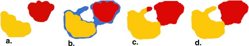
User interaction
Get Radiology Tree app to read full this article<
Get Radiology Tree app to read full this article<
Get Radiology Tree app to read full this article<
Get Radiology Tree app to read full this article<
Get Radiology Tree app to read full this article<
Get Radiology Tree app to read full this article<
Get Radiology Tree app to read full this article<
DSC=2×MAN∩SAM(MAN+SAM), DSC
=
2
×
MAN
∩
SAM
(
MAN
+
SAM
)
,
where MAN denotes the voxels segmented manually and SAM the voxels segmented semiautomatically. A DSC of 1 means 100% congruency; no congruency will result in a DSC of 0. There is no common agreement on a minimum value for an acceptable DSC, but coefficients > 0.7 have been considered good or high in previous publications .
Get Radiology Tree app to read full this article<
Get Radiology Tree app to read full this article<
Results
Manual Segmentation
Get Radiology Tree app to read full this article<
Get Radiology Tree app to read full this article<
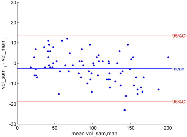
![Figure 5, (a) Intrarater reliability for manual segmentation in a subset of n = 18. Each point represents one magnetic resonance (MR) image in which the demyelination load was determined manually twice by the same rater (P.C.), showing in a Bland-Altman plot the mean volume of the two measures on the x axis and the difference between them on the y axis. (b) Intrarater reliability for semiautomated segmentation in a subset of n = 18 (same images as in [a]). Each point represents one MR image in which the demyelination load was determined semiautomatically twice by the same rater (P.C.). (c) Interrater reliability for manual segmentation in a subset of n = 18 (same images as in [a]). Each point represents one MR image in which the demyelination load was determined manually twice, once by P.C. and once by S.G. (d) Interrater reliability for semiautomated segmentation in a subset of n = 18 (same images as in [a]). Each point represents one MR image in which the demyelination load was determined semiautomatically twice, once by P.C. and once by S.G.](https://storage.googleapis.com/dl.dentistrykey.com/clinical/ASemiAutomaticAlgorithmforDeterminingtheDemyelinationLoadinMetachromaticLeukodystrophy/4_1s20S1076633211004375.jpg)
Get Radiology Tree app to read full this article<
Get Radiology Tree app to read full this article<
Semiautomatic Segmentation
Get Radiology Tree app to read full this article<
Get Radiology Tree app to read full this article<
Get Radiology Tree app to read full this article<
Get Radiology Tree app to read full this article<
Comparison between Manual and Semiautomatic Segmentation
Get Radiology Tree app to read full this article<
Get Radiology Tree app to read full this article<
Discussion
Get Radiology Tree app to read full this article<
Get Radiology Tree app to read full this article<
Get Radiology Tree app to read full this article<
Get Radiology Tree app to read full this article<
Get Radiology Tree app to read full this article<
Get Radiology Tree app to read full this article<
Get Radiology Tree app to read full this article<
Get Radiology Tree app to read full this article<
Get Radiology Tree app to read full this article<
Get Radiology Tree app to read full this article<
Get Radiology Tree app to read full this article<
Get Radiology Tree app to read full this article<
Conclusions
Get Radiology Tree app to read full this article<
Acknowledgments
Get Radiology Tree app to read full this article<
Get Radiology Tree app to read full this article<
References
1. Gieselmann V., Krageloh-Mann I.: Metachromatic leukodystrophy—an update. Neuropediatrics 2010; 41: pp. 1-6.
2. Kehrer C., Blumenstock G., Gieselmann V., et. al.: The natural course of gross motor deterioration in Metachromatic leukodystrophy. Dev Med Child Neurol 2011; 53: pp. 850-855.
3. Biffi A., Lucchini G., Rovelli A., et. al.: Metachromatic leukodystrophy: an overview of current and prospective treatments. Bone Marrow Transplant 2008; 42: pp. S2-S6.
4. Eichler F., Grodd W., Grant E., et. al.: Metachromatic leukodystrophy: a scoring system for brain MR imaging observations. AJNR Am J Neuroradiol 2009; 30: pp. 1893-1897.
5. Groeschel S., Kehrer C., Engel C., et. al.: Metachromatic leukodystrophy: natural course of cerebral MRI changes in relation to clinical course. J Inherit Metab Dis 2011; 34: pp. 1095-1102.
6. Filippi M., Horsfield M.A., Tofts P.S., et. al.: Quantitative assessment of MRI lesion load in monitoring the evolution of multiple sclerosis. Brain 1995; 118: pp. 1601-1612.
7. Paty D.W., Li D.K., Oger J.J., et. al.: Magnetic resonance imaging in the evaluation of clinical trials in multiple sclerosis. Ann Neurol 1994; 36: pp. S95-S96.
8. Paty D.W., Li D.K., UBC MS/MRI Study Group and the IFNB Multiple Sclerosis Study Group: Interferon beta-1b is effective in relapsing-remitting multiple sclerosis. II. MRI analysis results of a multicenter, randomized, double-blind, placebo-controlled trial. Neurology 1993; 43: pp. 662-667.
9. Fazekas F., Soelberg-Sorensen P., Comi G., et. al.: MRI to monitor treatment efficacy in multiple sclerosis. J Neuroimaging 2007; 17: pp. 50S-55S.
10. Seghier M.L., Ramlackhansingh A., Crinion J., et. al.: Lesion identification using unified segmentation-normalisation models and fuzzy clustering. Neuroimage 2008; 41: pp. 1253-1266.
11. Rorden C., Karnath H.O.: Using human brain lesions to infer function: a relic from a past era in the fMRI age?. Nat Rev Neurosci 2004; 5: pp. 813-819.
12. i Dali C., Hanson L.G., Barton N.W., et. al.: Brain N-acetylaspartate levels correlate with motor function in metachromatic leukodystrophy. Neurology 2010; 75: pp. 1896-1903.
13. Yushkevich P.A., Piven J., Hazlett H.C., et. al.: User-guided 3D active contour segmentation of anatomical structures: significantly improved efficiency and reliability. Neuroimage 2006; 31: pp. 1116-1128.
14. Bleau A., Leon L.J.: Watershed-based segmentation and region merging. Comput Vis Image Und 2000; 77: pp. 317-370.
15. Otsu N.: A threshold selection method from gray-level histograms. IEEE Trans Syst Man Cybernet 1979; 9: pp. 62-66.
16. Bland J.M., Altman D.G.: Statistical methods for assessing agreement between 2 methods of clinical measurement. Lancet 1986; 1: pp. 307-310.
17. Zou K.H., Warfield S.K., Bharatha A., et. al.: Statistical validation of image segmentation quality based on a spatial overlap index. Acad Radiol 2004; 11: pp. 178-189.
18. Garcia-Lorenzo D., Lecoeur J., Arnold D.L., et. al.: Multiple sclerosis lesion segmentation using an automatic multimodal graph cuts. Med Image Comput Comput Assist Interv 2009; 12: pp. 584-591.
19. Minamikawa-Tachino R., Maeda Y., Fujishiro I., et. al.: Three-dimensional brain visualization for metachromatic leukodystrophy. Brain Dev 1996; 18: pp. 394-399.
20. Wilke M., de Haan B., Juenger H., et. al.: Manual, semi-automated, and automated delineation of chronic brain lesions: a comparison of methods. Neuroimage 2011; 56: pp. 2038-2046.
21. Wilke M., Holland S.K.: Variability of gray and white matter during normal development: a voxel-based MRI analysis. Neuroreport 2003; 14: pp. 1887-1890.
22. Sharma N., Aggarwal L.M.: Automated medical image segmentation techniques. J Med Phys 2010; 35: pp. 3-14.
23. Ashburner J., Friston K.J.: Unified segmentation. Neuroimage 2005; 26: pp. 839-851.
24. Wang H., Chen X., Moss R.H., et. al.: Watershed segmentation of dermoscopy images using a watershed technique. Skin Res Technol 2010; 16: pp. 378-384.
25. Letteboer M.M., Olsen O.F., Dam E.B., et. al.: Segmentation of tumors in magnetic resonance brain images using an interactive multiscale watershed algorithm. Acad Radiol 2004; 11: pp. 1125-1138.
26. Kass M., Witkin A., Terzopoulos D.: Snakes—active contour models. Int J Comput Vision 1987; 1: pp. 321-331.
27. Joe B.N., Fukui M.B., Meltzer C.C., et. al.: Brain tumor volume measurement: comparison of manual and semiautomated methods. Radiology 1999; 212: pp. 811-816.
28. Schenk A., Prause G., Peitgen H.O.: Efficient semiautomatic segmentation of 3D objects in medical images. Lect Notes Comput Sci 2000 1935; pp. 186-195.
29. Kloppel S., Abdulkadir A., Hadjidemetriou S., et. al.: A comparison of different automated methods for the detection of white matter lesions in MRI data. Neuroimage 2011; 57: pp. 416-422.
30. Majumdar S., Orphanoudakis S.C., Gmitro A., et. al.: Errors in the measurements of T2 using multiple-echo MRI techniques. II. Effects of static field inhomogeneity. Magn Reson Med 1986; 3: pp. 562-574.
31. Rorden C., Karnath H.O., Bonilha L.: Improving lesion-symptom mapping. J Cogn Neurosci 2007; 19: pp. 1081-1088.
32. Ashburner J., Friston K.J.: Voxel-based morphometry—the methods. Neuroimage 2000; 11: pp. 805-821.
33. Valdés Hernandez M.C., Ferguson K.J., Chappell F.M., et. al.: New multispectral MRI data fusion technique for white matter lesion segmentation: method and comparison with thresholding in FLAIR images. Eur Radiol 2010; 20: pp. 1684-1691.
34. Schnack H.G., van Haren N.E., Brouwer R.M., et. al.: Mapping reliability in multicenter MRI: voxel-based morphometry and cortical thickness. Hum Brain Mapp 2010; 31: pp. 1967-1982.