Accuracy Evaluation of Automatic Quantification of the Articular Cartilage Surface Curvature from MRI

Rationale and Objectives

To study the articular cartilage surface curvature determined automatically from magnetic resonance (MR) knee scans, evaluate accuracy of the curvature estimates on digital phantoms, and an evaluation of their potential as disease markers for different stages of osteoarthritis (OA).

Materials and Methods

Knee MR data were acquired using a low-field 0.18T scanner, along with posteroanterior x-rays for evaluation of radiographic signs of OA according to the Kellgren-Lawrence index (KL). Scans from a total of 114 knees from test subjects with KL 0–3, 59% females, ages 21–79 years were evaluated. The surface curvature for the medial tibial compartment was estimated automatically on a range of scales by two different methods: Euclidean shortening flow and boundary normal comparison on a cartilage shape model. The curvature estimates were normalized for joint size for intersubject comparisons. Digital phantoms were created to establish the accuracy of the curvature estimation methods.

Results

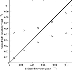
A comparison of the two curvature estimation methods to ground truth yielded absolute pairwise differences of 1.1%, and 4.8%, respectively. The interscan reproducibility for the two methods were 2.3% and 6.4% (mean coefficient of variation), respectively. The surface curvature was significantly higher in the OA population (KL > 0) compared with the healthy population (KLi = 0) for both curvature estimates, with P values of .000004 and .000006, respectively. The shape model based curvature estimate could also separate healthy from borderline OA (KL = 1) populations ( P = .005).

Conclusion

The phantom study showed that the shape model method was more accurate for a coarse-scale analysis, whereas the shortening flow estimated fine scales better. Both the fine- and the coarse-scale curvature estimates distinguished between healthy and OA populations, and the coarse-scale curvature could even distinguish between healthy and borderline OA populations. The highly significant differences between populations demonstrate the potential of cartilage curvature as a disease marker for OA.

Osteoarthritis (OA) is a disease characterized by degeneration of the articular cartilage and bone deformations in joints, is second to heart disease in causing work disability, and is associated with a large socioeconomic impact on health care systems ( ). Even though much effort has focused on development of disease modifying OA drugs, there is no standard clinical treatment of OA that can reverse cartilage degeneration. In clinical studies of new treatments, the ability to detect even small differences across populations receiving treatment or placebo could significantly reduce the cost of such studies. If OA can be detected at an early stage, patients that would be benefit from non medicinal intervention such as gait adjustment could be identified. Hence reliability and early OA detection are desirable features for OA disease markers.

Radiographs currently present the gold standard for measuring cartilage degradation in terms of joint space narrowing, and for determining the degree of OA using the Kellgren-Lawrence index (KL) ( ). However, standard radiographs are limited to a two-dimensional (2D) analysis of the joint and only measures the cartilage indirectly because it is not visible in the images. It is also sensitive to malpositioning, exposes test subjects to radiation, and is insensitive to small changes in the cartilage structure. Magnetic resonance imaging (MRI) has become one of the leading imaging modalities in osteoarthritis research because it allows for noninvasive, three-dimensional (3D) quantification of the articular cartilage ( ). Typical quantitative disease markers from MRI are the articular cartilage volume and thickness ( ) in which the volume on its own can be a relatively poor disease marker ( ).

Get Radiology Tree app to read full this article<

Materials and methods

Population and Image Acquisition

Get Radiology Tree app to read full this article<

Cartilage Segmentation

Get Radiology Tree app to read full this article<

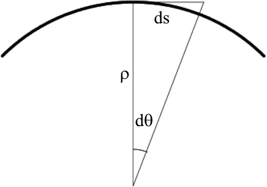
Curvature Estimation

Get Radiology Tree app to read full this article<

Curvature Analysis by Shortening Flow

Get Radiology Tree app to read full this article<

t=κM|∇|=[∇(∇|∇|)]|∇|, t

∇

[

∇

(

∇

)

]

∇

where ∇ϕ is the gradient of the level set representation ϕ, and the mean curvature can be written

κM=(2x(yy+zz)+2y(xx+zz)+2z(xx+yy)−2(xyxy+xzxz+yzyz))/(2(2x+2y+2z))3/2 κ

(

⁢

)

(

⁢

)

(

⁢

)

−

(

⁢

)

(

)

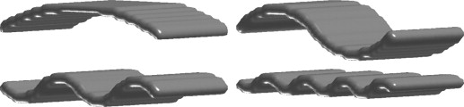
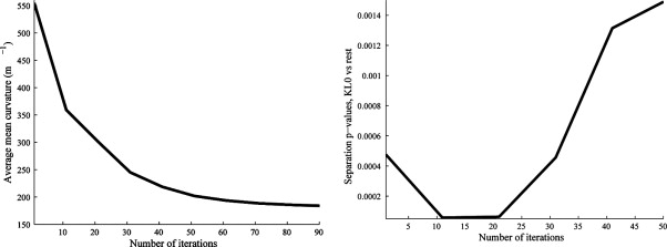
in terms of derivatives of ϕ. The average mean curvature on the articular surface was calculated throughout the evolution and curvature estimates at the point during the flow that enables best separation between groups as described in Differentiation Between Populations and elsewhere ( ). The supersampling, making 5 × 5 × 5 voxels from each voxel before the evolution, was done to allow finer changes than the original voxel size. There was no smoothing involved in the supersampling, so the shortening flow will initially mainly reduce partial volume effects because it can be considered as a nonlinear smoothing process. In late stages of the flow, the object loses its cartilage like form and may even change topology. Figure 2 illustrates how a cartilage sheet deforms during mean curvature flow.

Get Radiology Tree app to read full this article<

Curvature Analysis by Shape Model

Get Radiology Tree app to read full this article<

Normalization of Curvature Estimates

Get Radiology Tree app to read full this article<

Analysis on Digital Phantoms

Get Radiology Tree app to read full this article<

Results

Evaluation on Phantoms

Get Radiology Tree app to read full this article<

Differentiation Between Populations

Get Radiology Tree app to read full this article<

Table 1

The Average Curvature Values for the Shortening Flow (Flow) and Shape Model (Shape) Curvature Estimation Methods in Different Populations Based on KL

Method KL = 0 KL = 1 KL = 2 KL = 3 Flow (m −1 ) 341 (± 29) 339 (± 29) 390 (± 46) 410 (± 46) Shape (m −1 ) 40 (± 5.4) 45 (± 7.3) 47 (± 7.1) 54 (± 13.6)

Values in parenthesis are standard deviations (SD).

KL: Kellgren-Lawrence index.

Table 2

Results Comparing the Performance of the Two Curvature Methods and Cartilage Volume and Thickness

Flow Shape Volume Thickness Average 360 (m −1 ) 45 (m −1 ) 1,900 (mm 3 ) 1.30 mm SD 32 (m −1 ) 9.6 (m −1 ) 440 (mm 3 ) 0.18 mm Maximum 465 (m −1 ) 100 (m −1 ) 3100 (mm 3 ) 1.70 mm Minimum 302 (m −1 ) 30 (m −1 ) 580 (mm 3 ) 0.79 mm Cartilage volume (%) 2.3 6.4 5.3 4.6 Diff (%) 3.3 9.0 7.5 6.4P (KL > 0) .00006 .000004 .004 .002P (KL > 1) .75 .005 .27 .32

Average curvature with standard deviation and maximum and minimum values are listed for the 114 evaluation scans, along with precision values, mean cartilage volume and absolute mean pairwise difference (diff), for the 31 scan-rescan pairs. P values for separation between the healthy population and osteoarthritis (OA) population (Kellgren-Lawrence index [KL] > 0) and borderline OA (KL = 1) are also listed.

Get Radiology Tree app to read full this article<

Discussion

Get Radiology Tree app to read full this article<

References

1. Jackson D., Simon T., Aberman H.: Symptomatic articular cartilage degeneration: the impact in the new millennium. Clin Orthop Related Res 2001; 391: pp. 14-25.
2. Kellgren J., Lawrence J.: Radiological assessment of osteo-arthrosis. Ann Rheum Dis 1957; 16: pp. 494-502.
3. Graichen H., Eisenhart-Rothe R.V., Vogl T., et. al.: Quantitative assessment of cartilage status in osteoarthritis by quantitative magnetic resonance imaging. Arthr Rheum 2004; 50: pp. 811-816.
4. Pessis E., Drape J.-L., Ravaud P., et. al.: Assessment of progression in knee osteoarthritis: results of a 1 year study comparing arthroscopy and MRI. Osteoarthr Cartilage 2003; 11: pp. 361-369.
5. Peterfy C., Gold G., Eckstein F., et. al.: MRI protocols for whole-organ assessment of the knee in osteoarthritis. Osteoarthr Cartilage 2006; 14: pp. 95-111.
6. Stammberger T., Eckstein F., Englmeier K.-H., et. al.: Determination of 3D cartilage thickness data from MR imaging: computational method and reproducibility in the living. Magnet Res Med 1999; 41: pp. 529-536.
7. Dam E.B., Folkesson J., Pettersen P., et. al.: Automatic cartilage thickness quantification using a statistical shape model.2006.
8. Solloway S., Hutchinson C., Vaterton J., et. al.: The use of active shape models for making thickness measurements of articular cartilage from MR images. Magn Res Med 1997; 37: pp. 943-952.
9. Lynch J.A., Zaim S., Zhao J., et. al.: Cartilage segmentation of 3d MRI scans of the osteoarthritic knee combining user knowledge and active contours. SPIE 2000; 3979: pp. 925-935.
10. Gandy S., Dieppe P., Keen M., et. al.: No loss of cartilage volume over three years in patients with knee osteoarthritis as assessed by magnetic resonance imaging. Osteoarthr Cartilage 2002; 10: pp. 929-937.
11. Bullough P.: The geometry of diarthrodial joints, its physiologic maintenance, and the possible significance of age related changes in geometry to load distribution and the development of osteoarthritis. Clin Orthop 1981; 156: pp. 61-66.
12. Mankin H., Dorfman H., Lipiella L., et. al.: Biochemical and metabolic abnormalities in articular cartilage from osteoarthritic human hips. J Bone Joint Surg Am 1971; 53: pp. 523-537.
13. Terukina M., Fujioka H., Yoshiya S., et. al.: Analysis of the thickness and curvature of articular cartilage of the femoral condyle. Arthroscopy 2003; 19: pp. 969-973.
14. Hohe J., Ateshian G., Reiser M., et. al.: Surface size, curvature analysis, and assessment of knee joint incongruity with MRI in vivo. Magnet Reson Med 2002; 47: pp. 554-561.
15. Zhao L., Botha C., Bescos J., et. al.: Lines of curvature for polyp detection in virtual colonoscopy. IEEE Trans Visual Comp Graphics 2006; 12: pp. 885-892.
16. van Vliet L., Verbeek P.: Curvature and bending energy in digitized 2D and 3D images.1993.pp. 1403-1410. Tromso, Norway
17. Dunn T., Lu Y., Jin H., et. al.: T2 relaxation time of cartilage at MR imaging: comparison with severity of knee osteoarthritis. Radiology 2004; 232: pp. 592-598.
18. Folkesson J., Dam E.B., Olsen O.F., et. al.: Segmenting articular cartilage automatically using a voxel classification approach. IEEE Trans Med Imaging 2007; 26: pp. 106-115.
19. Kimmel R.: Numerical geometry of images: theory, algorithms and applications.2000.Springer, VerlagNew York:
20. Osher S., Fedkiw R.: Level set methods and dynamic implicit surfaces, vol. 153.2003.Springer, VerlagNew York
21. Sethian J.: Level set methods and fast marching methods.1999.Cambridge University PressCambridge, UK:
22. Folkesson J., Dam E.B., Olsen O.F., et. al.: Automatic curvature analysis of the articular cartilage surface.2006.
23. Pizer S.M., Fletcher P.T., Joshi S., et. al.: Deformable m-reps for 3d medical image segmentation. International Journal on Computer Vision 2003; pp. 85-106.

Accuracy Evaluation of Automatic Quantification of the Articular Cartilage Surface Curvature from MRI

Rationale and Objectives

Materials and Methods

Results

Conclusion

Materials and methods

Population and Image Acquisition

Cartilage Segmentation

Curvature Estimation

Curvature Analysis by Shortening Flow

Curvature Analysis by Shape Model

Normalization of Curvature Estimates

Analysis on Digital Phantoms

Results

Evaluation on Phantoms

Differentiation Between Populations

Discussion

References

Further Reading

3D Shape Analysis of the Supraspinatus Muscle

A Computer-Based Radiology Simulator as a Learning Tool to Help Prepare First-Year Residents for Being On Call

A Review of Research Into the Development of Radiologic Expertise Implications for Computer-Based Training