Accurate Prostate Volume Estimation Using Multifeature Active Shape Models on T2-weighted MRI

Rationale and Objectives

Accurate prostate volume estimation is useful for calculating prostate-specific antigen density and in evaluating posttreatment response. In the clinic, prostate volume estimation involves modeling the prostate as an ellipsoid or a spheroid from transrectal ultrasound, or T2-weighted magnetic resonance imaging (MRI). However, this requires some degree of manual intervention, and may not always yield accurate estimates. In this article, we present a multifeature active shape model (MFA) based segmentation scheme for estimating prostate volume from in vivo T2-weighted MRI.

Materials and Methods

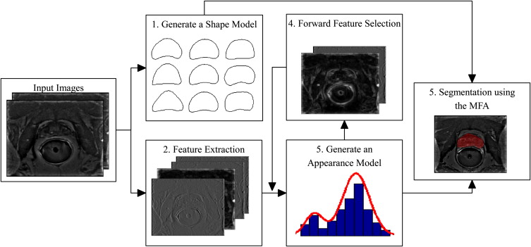
We aim to automatically determine the location of the prostate boundary on in vivo T2-weighted MRI, and subsequently determine the area of the prostate on each slice. The resulting planimetric areas are aggregated to yield the volume of the prostate for a given patient. Using a set of training images, the MFA learns the most discriminating statistical texture descriptors of the prostate boundary via a forward feature selection algorithm. After identification of the optimal image features, the MFA is deformed to accurately fit the prostate border. An expert radiologist segmented the prostate boundary on each slice and the planimetric aggregation of the enclosed areas yielded the ground truth prostate volume estimate. The volume estimation obtained via the MFA was then compared against volume estimations obtained via the ellipsoidal, Myschetzky, and prolated spheroids models.

Results

We evaluated our MFA volume estimation method on a total 45 T2-weighted in vivo MRI studies, corresponding to both 1.5 Tesla and 3.0 Tesla field strengths. The results revealed that the ellipsoidal, Myschetzky, and prolate spheroid models overestimated prostate volumes, with volume fractions of 1.14, 1.53, and 1.96, respectively. By comparison, the MFA yielded a mean volume fraction of 1.05, evaluated using a fivefold cross-validation scheme. A correlation with the ground truth volume estimations showed that the MFA had an r 2 value of 0.82, whereas the clinical volume estimation schemes had a maximum value of 0.70.

Conclusions

Our MFA scheme involves minimal user intervention, is computationally efficient and results in volume estimations more accurate than state of the art clinical models.

Prostate volume has been shown to be a strong predictor of treatment outcome for patients with prostate cancer , especially when combined with a baseline prostate-specific antigen (PSA) level . Prostate volume has also been shown to be useful in determining PSA density . The most common method for estimating the prostate volume involves modeling the prostate as a simple geometric shape based on manually estimated measurements of the anteroposterior, transverse, and craniocaudal lengths of the prostate.

The most common models for approximating the prostate shape are the ellipsoid model and the prolate spheroid model . It is important to note that the ellipsoidal model has been a clinical standard for comparisons from at least 1991 to the present day . Some researchers have reported that in several cases the ellipsoid model underestimated the prostate volume . Tewari et al and Eri et al both found that the ellipsoid model underestimated the prostate volume by about 10%. Matthews et al found that the ellipsoid model from transrectal ultrasound (TRUS) imagery underestimated the volume for large prostates (>50 mL), but overestimated the volume for small prostates (<30 mL). Myschetzky et al overcame this underestimation by proposing a new formula in which the ellipsoid volume estimation is multiplied by a factor of 1.34 . Additionally, methods involving manual intervention are typically subject to inter- and intraobserver variability and these volume estimations are not highly reproducible.

Get Radiology Tree app to read full this article<

Materials and methods

Data Description and Notation

Get Radiology Tree app to read full this article<

Table 1

Data Description

Dataset Field Strength Total Studies Slice ( M ) per Study_X-Y_ Dimensions_T_ (mm) Pixels mm D 1 1.5 Tesla 19 10 ≤ M ≤ 17 256 × 256 140 × 140 3.0 D 2 3.0 Tesla 26 8 ≤ M ≤ 20 512 × 512 140 × 140 2.2

Get Radiology Tree app to read full this article<

Ground Truth Estimations of Prostate Volume

Get Radiology Tree app to read full this article<

VEx=T⋅∑Mm=1Am. V

∑

Get Radiology Tree app to read full this article<

Clinically Employed Prostate Volume Estimation Models

Get Radiology Tree app to read full this article<

Table 2

Enumeration of Prostate Volume Estimation Techniques Employed in this Article with Corresponding Formulae

Experiment Description Model_V__ϵ 1_ Ellipsoid_Ell__D_ 1 · D 2 · D 3 · π/6ϵ 2 Myschetzky_Mys__D_ 1 · D 2 · D 3 · 0.7ϵ 3 Prolate spheroid_Sph_ ( D 1 ) 2 · D 2 · π/6ϵ 4 Multifeature ASM_MFA_T⋅∑Mm=1Am T

∑

m Expert_Ex_T⋅∑Mm=1Am T

∑

Get Radiology Tree app to read full this article<

MFA-based Prostate Volume Estimations (V MFA )

Get Radiology Tree app to read full this article<

Generating a statistical shape model

Get Radiology Tree app to read full this article<

Feature extraction

Get Radiology Tree app to read full this article<

Generate an appearance model

Get Radiology Tree app to read full this article<

Forward feature selection

Get Radiology Tree app to read full this article<

Segmentation using the MFA

Get Radiology Tree app to read full this article<

Experiments Performed

Get Radiology Tree app to read full this article<

Results

Pearson’s Correlation Coefficient

Get Radiology Tree app to read full this article<

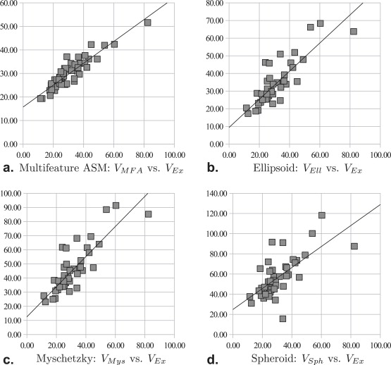
Table 3

Pearson’s Correlation Coefficient ( r 2 ) between V and V Ex over 45 Studies

Model_V Ell__V Mys__V Sph__V MFA__r 2_ 0.700 0.700 0.454 0.823

Get Radiology Tree app to read full this article<

Comparison of Volume Fractions

Get Radiology Tree app to read full this article<

Table 4

Comparison of V / V Ex in Terms of Mean, Standard Deviation (SD), and Standard Error (STE) over 45 Studies

Experiment_V_ Mean SD STE_ϵ 1_V Ell 1.143 0.252 0.0376ϵ 2 V Mys 1.528 0.337 0.0502ϵ 3 V Sph 1.958 0.587 0.0875ϵ 4 V MFA 1.053 1.207 0.0277

Get Radiology Tree app to read full this article<

Statistical Significance Between Volume Fractions

Get Radiology Tree app to read full this article<

Table 5

P Values from Each Set of Paired Student t -tests Between V MFA / V Ex and V Ell / V Ex , V Mys / V Ex , V Sph / V Ex over 45 Studies

V Ell /V Ex__V Mys /V Ex__V Sph /V Ex__V Mys /V Ex 4.33 × 10 –2 ∗ 2.01 × 10 –12 ∗∗ 7.85 × 10 –16 ∗∗

Get Radiology Tree app to read full this article<

Discussion

Get Radiology Tree app to read full this article<

Acknowledgments

Get Radiology Tree app to read full this article<

Appendix

Multifeature active shape model

Input Training Images

Get Radiology Tree app to read full this article<

Generate a Shape Model

Get Radiology Tree app to read full this article<

X=X¯¯¯+P⋅b, X

⋅

where X¯¯¯ X

¯ represents the mean shape, P is a matrix of the first few principal components (Eigenvectors) of the shape obtained via principal component analysis (PCA), and b is a vector defining the shape, where the individual elements of b can range between –3 and +3 standard deviations from the mean shape X¯¯¯ X

¯ . In our training stage, we have equally spaced 100 landmarks ( N = 100) along the prostate boundary in each slice, and have aligned the landmarks by selecting the topmost landmark in each image as landmark #1.

Get Radiology Tree app to read full this article<

Extract Features

Get Radiology Tree app to read full this article<

k1=⎡⎣⎢5−3−350−35−3−3⎤⎦⎥,k5=⎡⎣⎢10−120−210−1⎤⎦⎥. k

[

−

]

[

−

]

Get Radiology Tree app to read full this article<

G(c)={g(c)⊗k1,…,g(c)⊗k14,xc,yc}. G

(

)

{

(

)

⊗

…

(

)

⊗

}

Get Radiology Tree app to read full this article<

Generate an Appearance Model

Get Radiology Tree app to read full this article<

μ,Σ,w=argmaxμ,Σ,w∑Tt=1(ln∑Qq=1wq⋅p(Gt|μq,∑q)). μ

arg

max

∑

(

∑

(

∑

)

Get Radiology Tree app to read full this article<

Segmenting an Image Using the MFA

Get Radiology Tree app to read full this article<

b=P′⋅(Xˆi−Xi) b

′

(

−

)

Get Radiology Tree app to read full this article<

Xˆ={en|en=argmaxd∈nκ(c)P(G(d)|μ,Σ,w),n∈{1,…,N}} X

{

arg

max

∈

(

)

(

)

∈

{

…

}

Get Radiology Tree app to read full this article<

Get Radiology Tree app to read full this article<## Forward Feature Selection

Get Radiology Tree app to read full this article<

Get Radiology Tree app to read full this article<## References

- 1. Pierorazio P., Kinnaman M., Wosnitzer M., et. al.: Prostate volume and pathologic prostate cancer outcomes after radical prostatectomy. Urology 2007; 70: pp. 696-701.

- 2. Kaminski J., Hanlon A., Horwitz E., et. al.: Relationship between prostate volume, prostate-specific antigen nadir, and biochemical control. Int J Radiat Oncol Biol Phys 2002; 5: pp. 888-892.

- 3. Roehrborn C., Boyle P., Bergner D., et. al.: Serum prostate-specific antigen and prostate volume predict long-term changes in symptoms and flow rate: results of a four-year, randomized trial comparing finasteride versus placebo. Adult Urol 1999; 54: pp. 662-670.

- 4. Bangma C., Niemer A., Grobbee D., et. al.: Transrectal ultrasonic volumetry of the prostate: in vivo comparison of different methods. Prostate 1966; 28: pp. 107-110.

- 5. Hoffelt S., Marshall L., Garzotto M., et. al.: A comparison of CT scan to transrectal ultrasound measured prostate volume in untreated prostate cancer. Int J Radiat Oncol Biol Phys 2003; 57: pp. 29-32.

- 6. Eri L., Thomassen H., Brennhovd B., et. al.: Accuracy and repeatability of prostate volume measurements by transrectal ultrasound. Nature 2002; 5: pp. 273-278.

- 7. Littrup P., Williams C., Egglin T., et. al.: Determination of prostate volume with transrectal us for cancer screening. Part 11. Accuracy of in vitro and in vivo techniques. Radiology 1991; 52: pp. 49-53.

- 8. Matthews G., Motta J., Fracchia J.: The accuracy of transrectal ultrasound prostate volume estimation: clinical correlations. J Clin Ultrasound 1996; 24: pp. 501-505.

- 9. Nathan M., Seenivasagam K., Mei Q., et. al.: Transrectal ultrasonography: why are estimates of prostate volume and dimension so inaccurate?. Br J Urol 1996; 77: pp. 401-407.

- 10. Park S., Kim J., Choi S., et. al.: Prostate volume measurements by TRUS using heights obtained by transaxial and midsagittal scanning: comparison with specimen volume following radical prostatectomy. Korean J Radiol 2000; 1: pp. 110-113.

- 11. Tewari R., Indudhara K., Shinohara E., et. al.: Comparison of transrectal ultrasound prostatic volume estimation with magnetic resonance imaging volume estimation and surgical specimen weight in patients with benign prostatic hyperplasia. J Clin Ultrasound 1996; 24: pp. 169-174.

- 12. Jeong C.W., Park H.K., Hong S.K., et. al.: Comparison of prostate volume measured by transrectal ultrasonography and MRI with the actual prostate volume measured after radical prostatectomy. Urol Int 2008; 81: pp. 179-185.

- 13. Sosna J., Rofsky N., Gaston S., et. al.: Determinations of prostate volume at 3-tesla using an external phased array coil: comparison to pathologic specimens. Acad Radiol 2003; 10: pp. 846-853.

- 14. MacMahon P., Kennedy A., Murphy D., et. al.: Modified prostate volume algorithm improves transrectal us volume estimation in men presenting for prostate brachytherapy. Radiology 2009; 250: pp. 273-280.

- 15. Myschetzky P., Suburu R., Kelly B.J., et. al.: Determination of prostate gland volume by transrectal ultrasound: correlation with radical prostatectomy specimens. Scand J Urol Nephrol Suppl 1991; 137: pp. 107-111.

- 16. Bonilla J., Stoner E., Grino P., et. al.: Intra- and interobserver variability of MRI prostate volume measurements. Prostate 1997; 31: pp. 98-102.

- 17. Aarnink R., de la Rosette J., Debruyne F., et. al.: Reproducibility of prostate volume measurements from transrectal ultrasonography by an automated and a manual technique. Br J Urol 1996; 78: pp. 219-223.

- 18. Cootes T., Taylor C., Cooper D., et. al.: Active shape models - their training and application. Comput Vision Image Understanding 1995; 61: pp. 38-59.

- 19. Seghers D., Loeckx D., Maes F., et. al.: Minimal shape and intensity cost path segmentation. IEEE Trans Med Imaging 2007; 26: pp. 1115-1129.

- 20. Madabhushi A., Udupa J.: Interplay of inhomogeneity correction and intensity standardization in MR image analysis. IEEE Trans Med Imaging 2005; 24: pp. 561-576.

- 21. Kirsch R.: Computer determination of the constituent structure of biological images. Comp Biomed Res 1971; 4: pp. 315-328.

- 22. Duda R., Hart P.: Pattern Classification and Scene Analysis.1973.John Wiley and Sons

- 23. Everitt B., Hand D.: Finite Mixture Distributions.1981.Chapman and HallLondon, UK

- 24. American College of Radiology Imaging Network. MR imaging and MR spectroscopic imaging of prostate cancer prior to radical prostatectomy: a prospective multi-institutional clinicopathological study. Available online at: www.acrin.org/Portals/0/Protocols/6659/A6659partial_summary.pdf

- 25. Edwards A. An Introduction to Linear Regression and Correlation. San Francisco: W.H. Freeman and Co Ltd, 1976; 33–46.

- 26. Ledoita O., Wolf M.: A well-conditioned estimator for large-dimensional covariance matrices. J Multivariate Anal 2004; 88: pp. 365-411.

- 27. Mahdavi S, Morris W, Spadinger I, et al. 3d prostate segmentation in ultrasound images based on tapered and deformed ellipsoids. In: MICCAI, vol. 12, Lecture Notes Comput Sci 960–967.

- 28. Dice L.: Measures of the amount of ecologic association between species. Ecology 1945; 263: pp. 297-302.

- 29. Klein S., van der Heide U., Lips I., et. al.: Automatic segmentation of the prostate in 3D MR images by atlas matching using localized mutual information. Med Phys 2008; 35: pp. 1407-1417.

- 30. Martin S., Daanen V., Troccaz J.: Automated segmentation of the prostate in 3d MR images using a probabilistic atlas and a spatially constrained deformable model. Med Phys 2010; 37: pp. 1579-1590.

- 31. Pasquier D., Lacornerie T., Vermandel M., et. al.: Automatic segmentation of pelvic structures from magnetic resonance images for prostate cancer radiotherapy. Int J Radiat Oncol Biol Phys 2007; 68: pp. 592-600.

- 32. Makni N., Puech P., Lopes R., et. al.: Combining a deformable model and a probabilistic framework for an automatic 3D segmentation of prostate on MRI. Int J CARS 2009; 4: pp. 181-188.

- 33. Guyon I., Elisseeff A.: An introduction to variable and feature selection. J Mach Learn Res 2003; 3: pp. 1157-1182.

Accurate Prostate Volume Estimation Using Multifeature Active Shape Models on T2-weighted MRI

Rationale and Objectives

Materials and Methods

Results

Conclusions

Materials and methods

Data Description and Notation

Ground Truth Estimations of Prostate Volume

Clinically Employed Prostate Volume Estimation Models

MFA-based Prostate Volume Estimations (V MFA )

Generating a statistical shape model

Feature extraction

Generate an appearance model

Forward feature selection

Segmentation using the MFA

Experiments Performed

Results

Pearson’s Correlation Coefficient

Comparison of Volume Fractions

Statistical Significance Between Volume Fractions

Discussion

Acknowledgments

Appendix

Multifeature active shape model

Input Training Images

Generate a Shape Model

Extract Features

Generate an Appearance Model

Segmenting an Image Using the MFA

Further Reading

Assessment of Left Ventricular Function and Mass by MR Imaging

Brain and Spine Imaging Patterns

Can Dual-energy CT Evaluate Contrast Enhancement of Ground-glass Attenuation?