Algorithm Variability in the Estimation of Lung Nodule Volume From Phantom CT Scans Results of the QIBA 3A Public Challenge

Rationale and Objectives

Quantifying changes in lung tumor volume is important for diagnosis, therapy planning, and evaluation of response to therapy. The aim of this study was to assess the performance of multiple algorithms on a reference data set. The study was organized by the Quantitative Imaging Biomarker Alliance (QIBA).

Materials and Methods

The study was organized as a public challenge. Computed tomography scans of synthetic lung tumors in an anthropomorphic phantom were acquired by the Food and Drug Administration. Tumors varied in size, shape, and radiodensity. Participants applied their own semi-automated volume estimation algorithms that either did not allow or allowed post-segmentation correction (type 1 or 2, respectively). Statistical analysis of accuracy (percent bias) and precision (repeatability and reproducibility) was conducted across algorithms, as well as across nodule characteristics, slice thickness, and algorithm type.

Results

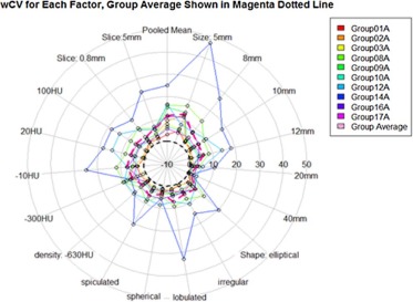
Eighty-four percent of volume measurements of QIBA-compliant tumors were within 15% of the true volume, ranging from 66% to 93% across algorithms, compared to 61% of volume measurements for all tumors (ranging from 37% to 84%). Algorithm type did not affect bias substantially; however, it was an important factor in measurement precision. Algorithm precision was notably better as tumor size increased, worse for irregularly shaped tumors, and on the average better for type 1 algorithms. Over all nodules meeting the QIBA Profile, precision, as measured by the repeatability coefficient, was 9.0% compared to 18.4% overall.

Conclusion

The results achieved in this study, using a heterogeneous set of measurement algorithms, support QIBA quantitative performance claims in terms of volume measurement repeatability for nodules meeting the QIBA Profile criteria.

Introduction

Because of the aggressive nature of lung cancer, the response of a patient to a particular treatment must be evaluated quickly and efficiently to get therapy started. X-ray computed tomography (CT) is an effective imaging technique for diagnosing lung tumors, planning therapy, and assessing therapy response. In clinical practice, qualitative impressions based on nothing more than visual inspection of the images are frequently sufficient for making patient management decisions. Quantification becomes helpful when tumor masses change slowly over the course of illness. Standards for measurement of objects within images are therefore a necessity to be able to help lung cancer patients. The Quantitative Imaging Biomarker Alliance (QIBA) has led this role, supported by the Radiological Society of North America (RSNA), as “an initiative by researchers, healthcare professionals, and industry to advance quantitative imaging and the use of imaging biomarkers in clinical trials and clinical practice.” 1

1 http://qibawiki.rsna.org .

The goal of the QIBA is to establish protocols and profiles (standards documents) that will lead to acceptance of quantitative imaging biomarkers by the imaging community, clinical trial industry, regulatory agencies, and clinicians, as reliable evidence of biology and pathophysiology. A QIBA Profile is a document that describes a specific performance claim and how it can be achieved. It is expected to provide specifications that may be adopted by users and equipment vendors to meet targeted levels of performance. The QIBA Profile for CT Tumor Volume Change can be found at http://www.rsna.org/QIBA_Protocols_and_Profiles.aspx .

Get Radiology Tree app to read full this article<

Materials and Methods

Participant Procedure

Get Radiology Tree app to read full this article<

Get Radiology Tree app to read full this article<

Get Radiology Tree app to read full this article< as described in the Protocol. QI-Bench provided resources that enabled better use of available data by providing data access methods and an analytical framework for evaluation and optimization. Get Radiology Tree app to read full this article<

Table 1

Number of Participants with Each Class by the Degree of Automation (Automation Class)

Automation Class Pilot ( n = 12) Pivotal ( n = 10) Semi-automatic type 1 6(50%) 4(40%) Semi-automatic type 2: limited parameter adjustment (on less than 15% of the cases) 1(8.3%) 1(10%) Semi-automatic type 2: moderate parameter adjustment (on less than 50% of the cases) 1(8.3%) 0 Semi-automatic type 2: extensive parameter adjustment (more than 50% of the cases) 0 1(10%) Semi-automatic type 2: limited image/boundary modification (on less than 15% of the cases) 0 0 Semi-automatic type 2: moderate image/boundary modification (on less than 50% of the cases) 1(8.3%) 1(10%) Semi-automatic type 2: extensive image/boundary modification (more than 50% of the cases) 0 1(10%) Unspecified 3(25%) 2(20%)

Get Radiology Tree app to read full this article<

Get Radiology Tree app to read full this article<

Get Radiology Tree app to read full this article<

Data Description

Get Radiology Tree app to read full this article<

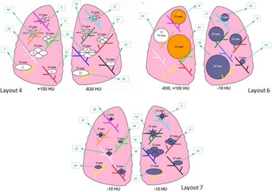
Table 2

Description of Data Used in the Study: Breakdown of Nodule Characteristics (Shape, Density, Size) and Slice Thickness

QIBA Type \* Lesion Type Slice Thickness (mm) 0.8 mm

QIBA Type = Yes 5.0 mm

QIBA Type = No No Spherical 5 mm, −10 HU 6 6 5 mm, 100 HU 2 2 8 mm, −10 HU 6 6 8 mm, 100 HU 2 2 20 mm, −630 HU 6 6 Elliptical 5 mm, −10 HU 6 6 8 mm, −10 HU 6 6 10 mm, −630 HU 6 6 20 mm, −630 HU 6 6 Lobulated 5 mm, −10 HU 6 6 8 mm, −10 HU 6 6 10 mm, −630 HU 6 6 20 mm, −630 HU 6 6 Spiculated 5 mm, −10 HU 6 6 8 mm, −10 HU 6 6 10 mm, −630 HU 6 6 20 mm, −630 HU 6 6 Irregular 8 mm, −300 HU 2 2 Yes Spherical 10 mm, −10 HU 6 6 10 mm, 100 HU 2 2 20 mm, −10 HU 6 6 20 mm, 100 HU 6 6 40 mm, −10 HU 6 6 40 mm, 100 HU 6 6 Elliptical 10 mm, −10 HU 6 6 10 mm, 100 HU 6 6 20 mm, −10HU 6 6 20 mm, 100 HU 6 6 Lobulated 10 mm, −10 HU 6 6 10 mm, 100 HU 6 6 20 mm, −10 HU 6 6 20 mm, 100 HU 6 6 Spiculated 10 mm, −10 HU 6 6 10 mm, 100 HU 6 6 20 mm, −10 HU 6 6 20 mm, 100 HU 6 6 Irregular 10 mm, 100 HU 2 2 12 mm, 20 HU 2 2 Total 204 204

QIBA, Quantitative Imaging Biomarker Alliance.

Notes: 8 mm of irregular lesion with −300 HU has only four scans of lesions, and 12 mm of irregular lesion with 20 HU has only four scans of lesions.

Get Radiology Tree app to read full this article<

Data Preparation

Get Radiology Tree app to read full this article<

Statistical Data Analysis

Get Radiology Tree app to read full this article<

%Biasjk={∑Ni=1∑Ll=1[(Yijkl−Xi)Xi]/(N×L)}×100. %

Bias

{

∑

[

(

ijkl

−

)

]

(

)

}

100

Get Radiology Tree app to read full this article<

Results

%Bias

Get Radiology Tree app to read full this article<

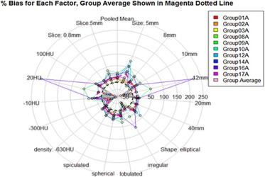
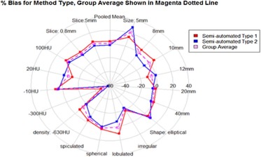
Table 3

Mean of %Bias and 95% CI of the Mean of %Bias as a Function of Nodule Characteristics and Reconstructed Slice Thickness

Parameter Value Semi-Automatic Type 1 Algorithm (%) Semi-Automatic Type 2 Algorithm (%) All (%) Shape Spherical 4.12 0.86 2.49 [2.77, 5.47] [−1.38, 3.17] [1.13, 3.83] Elliptical 5.28 9.54 7.41 [3.14, 7.33] [2.86, 16.28] [4.09, 10.71] Lobulated 10.78 −6.89 1.95 [8.05, 13.3] [−9.37, −4.37] [0.02, 3.83] Spiculated −2.29 −7.99 −5.14 [−4.28, −0.28] [−10.66, −5.39] [−6.72, −3.43] Irregular −18.79 −22.70 −20.74 [−28.95, −8.86] [−39.96, −5.5] [−30.96, −10.27] Density (HU) −630 \* −8.37 −19.44 −13.9 [−9.58, −7.12] [−20.79, −18.06] [−14.88, −12.93] −300 −47.88 −57.24 −52.56 [−58.04, −37.58] [−63.42, −50.83] [−59.32, −45.81] −10 8.84 5.11 6.97 [7.14, 10.53] [1.7, 8.53] [5.07, 8.78] 20 −11.02 −0.24 −5.63 [−33.31, 11.95] [−49.73, 50.53] [−32.48, 21.3] 100 6.05 1.15 3.60 [4.71, 7.35] [−1.11, 3.3] [2.23, 4.91] Slice thickness (mm) 5 \* 6.65 0.64 3.65 [4.71, 8.57] [−1.65, 2.93] [2.18, 5.16] 0.8 0.91 −4.04 −1.57 [−0.01, 1.83] [−7.26, −0.8] [−3.2, 0.1] Size (mm) 5 \* 13.77 28.67 21.22 [8.31, 19.14] [16.37, 40.98] [14.24, 28.09] 8 \* 4.91 −5.18 −0.14 [1.63, 8.18] [−8.79, −1.45] [−2.71, 2.44] 10 6.51 −7.92 −0.71 [4.74, 8.26] [−9.86, −5.92] [−2.13, 0.65] 12 −11.02 −0.24 −5.63 [−33.15, 1.28] [−49.88, 50.49] [−32.25, 20.54] 20 −1.76 −5.58 −3.67 [−2.45, −1.11] [−7.2, −3.97] [−4.58, −2.81] 40 0.67 −3.11 −1.22 [0.18, 1.18] [−4.58, −1.62] [−2.05, −0.36] All 3.78 −1.70 1.04 [2.68, 4.88] [−3.67, 0.28] [−0.06, 2.13]

Note: Results are tabulated across semi-automated type 1 and semi-automated type 2 algorithms.

Get Radiology Tree app to read full this article<

Table 4

Using Only the Nodules That Meet the QIBA CT Profile, the Mean of %Bias Estimates as a Function of Nodule Characteristics, and Reconstructed Slice Thickness

Shape Parameter Size, HU Parameters Semi-Automatic Type 1 Algorithm (%) Semi-Automatic Type 2 Algorithm (%) All (%) Spherical 10 mm, −10 HU 3.07 3.72 3.39 [−0.08, 6.21] [0.56, 6.88] [1.15, 5.63] 10 mm, 100 HU \* 1.36 −4.57 −1.60 [−2.74, 5.46] [−12.34, 3.21] [−6.21, 3.01] 20 mm, −10 HU 2.35 −2.95 −0.30 [1.20, 3.49] [−4.96, −0.94] [−1.71, 1.11] 20 mm, 100 HU 3.73 −2.11 0.81 [2.51, 4.95] [−3.65, −0.56] [−0.37, 1.99] 40 mm, −10 HU 0.19 −3.26 −1.54 [−0.43, 0.81] [−4.21, −2.31] [−2.28, −0.79] 40 mm, 100 HU 1.56 −0.28 0.64 [−0.88, 2.24] [−1.65, 1.09] [−0.16, 1.45] Elliptical 10 mm, −10 HU 9.34 −1.62 3.86 [7.14, 11.54] [−5.62, 2.38] [1.24, 6.49] 10 mm, 100 HU 11.36 4.86 8.11 [3.81, 18.91] [−2.82, 12.53] [2.63, 13.8] 20 mm, −10 HU .73 −5.54 −1.41 [1.68, 3.78] [−8.10, −2.99] [−3.14, 0.33] 20 mm, 100 HU 6.66 20.03 13.34 [5.56, 7.76] [6.99, 33.08] [6.65, 20.04] Lobulated 10 mm, −10 HU 8.60 −25.10 −8.25 [5.34, 11.86] [−37.87, −12.33] [−15.90, −0.60] 10 mm, 100 HU 4.73 0.0008 2.36 [2.25, 7.21] [−4.03, 4.03] [−0.08, 4.81] 20 mm, −10 HU 0.47 −2.13 −0.83 [−4.22, 5.17] [−4.30, 0.03] [−3.39, 1.73] 20 mm, 100 HU 3.53 −3.06 0.23 [2.22, 4.84] [−4.83, −1.29] [−1.14, 1.61] Spiculated 10 mm, −10 HU −5.15 −10.42 −7.78 [−6.86, −3.43] [−16.16, −4.68] [−10.84, −4.73] 10 mm, 100 HU −2.00 −8.67 −5.34 [−4.12, 0.11] [−11.86, −5.49] [−7.45, −3.23] 20 mm, −10 HU −1.76 −5.58 −4.94 [−2.45, −1.11] [−7.2, −3.97] [−6.85,−3.03] 20 mm, 100 HU −2.90 −6.95 −4.92 [−4.36, −1.44] [−11.82, −2.07] [−7.57, −2.28] Irregular 10 mm, 100 HU −2.10 −9.11 −5.60 [−5.21, 1.01] [−14.44, −3.77] [−8.96, −2.25] 12 mm, 20 HU \* −28.90 −11.50 −20.20 [−36.94, −20.85] [−72.52, 49.52] [−49.63, 9.24] All 1.89 −3.19 −0.65 [1.05, 2.72] [−5.04, −1.33] [−1.66, 0.36]

CT, computed tomography; QIBA, Quantitative Imaging Biomarker Alliance.

Note: Results are tabulated across five semi-automated type 1and 5 semi-automated type 2 algorithms.

Get Radiology Tree app to read full this article<

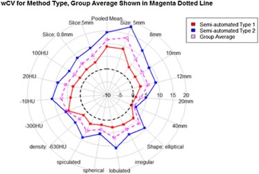
wCV

Get Radiology Tree app to read full this article<

Table 5

Estimated Coefficient of Variation (wCV) as a Function of Nodule Characteristics and Reconstructed Slice Thickness

Parameter Value Slice Thickness 0.8 mm (%) Slice Thickness 5 mm \* (%) All (%) Shape Spherical 3.69 4.54 4.11 [2.60, 4.77] [3.20, 5.87] [3.28, 4.94] Elliptical 5.19 7.82 6.50 [2.09, 8.28] [3.72, 11.91] [3.94, 9.07] Lobulated 7.89 6.28 7.08 [1.49, 14.29] [2.54, 10.01] [4.94, 10.96] Spiculated 4.77 7.35 6.06 [1.99, 7.54] [2.45, 12.26] [3.23, 8.89] Irregular 6.47 4.48 5.48 [3.08, 9.85] [0.61, 8.35] [2.90, 8.05] Density (HU) −630 \* 3.83 4.16 4.00 [2.89, 4.77] [3.07, 5.25] [3.24, 4.76] −300 8.80 3.75 6.27 [4.16, 13.44] [0.70, 7.43] [3.01, 9.54] −10 6.81 7.64 7.23 [3.07, 10.55] [4.60, 10.68] [4.66, 9.79] 20 6.11 6.00 6.06 [1.91, 10.32] [−0.68, 12.69] [2/17, 9.94] 100 3.76 5.51 4.64 [1.49, 6.03] [1.99, 9.04] [2.37, 6.91] Size (mm) 5 \* 13.10 12.35 12.73 [4.46, 21.74] [ 8.34, 16.36] [7.89, 17.55] 8 \* 7.56 7.41 7.49 [3.87, 11.25] [4.08, 10.74] [4.89, 10.08] 10 4.70 6.47 5.59 [3.14, 6.27] [4.03, 8.92] [4.12, 7.05] 12 6.11 6.00 6.06 [2.46, 9.77] [−0.27, 12.29] [2.63, 9.48] 20 2.30 3.53 2.91 [0.95, 3.65] [0.71, 6.34] [1.40, 4.43] 40 0.82 1.34 1.08 [0.32, 1.32] [0.63, 2.04] [0.65, 1.51] All 5.33 6.18 5.76 [4.08, 6.59] [5.15, 7.21] [4.93, 6.59]

Get Radiology Tree app to read full this article<

TDI 95%

Get Radiology Tree app to read full this article<

Table 6

TDI 95% by Nodule and Imaging Characteristics

Parameter Value Slice Thickness 0.8 mm (%) Slice Thickness 5 mm \* (%) All (%) Shape Spherical 23.83 70.02 54.26 [18.87, 28.80] [61.50, 78.54] [44.78, 63.74] Elliptical 43.27 70.84 44.92 [16.70, 69.83] [51.91, 89.76] [66.49, 66.06] Lobulated 49.05 64.86 62.75 [19.30, 78.79] [39.87, 89.84] [37.76, 87.74] Spiculated 33.08 62.13 51.91 [22.07, 44.08] [43.29, 80.97] [31.26, 72.55] Irregular 83.11 127.43 84.95 [3.62, 162.61] [−16.87, 271.73] [−2.69, 172.58] Density (HU) −630 \* 31.80 42.59 40.57 [30.28, 33.32] [41.18, 44.00] [25.95, 55.19] −300 83.11 72.33 78.97 [75.45, 90.77] [65.06, 79.60] [61.86, 96.08] −10 48.76 75.91 72.47 [33.42, 64.09] [69.77, 82.04] [57.58, 87.36] 20 165.12 263.19 188.14 [65.23, 265.01] [136.56, 389.83] [73.68, 302.60] 100 26.25 53.27 43.63 [21.74, 30.76] [44.32, 62.23] [36.6, 50.62] Size (mm) 5 \* 93.79 125.55 113.75 [23.92, 163.67] [84.13, 166.98] [69.68, 157.81] 8 \* 64.39 68.64 68.08 [48.63, 51.24] [59.25, 78.03] [46.90, 89.24] 10 31.74 63.75 51.91 [28.34, 35.14] [52.00, 75.49] [30.09, 73.72] 12 165.12 263.19 188.14 [66.89, 263.35] [134.65, 391.73] [68.72, 307.56] 20 21.51 32.30 27.50 [17.74, 25.28] [24.21, 40.40] [6.67, 48.33] 40 6.07 23.41 15.30 [4.77, 7.38] [19.92, 26.89] [4.98, 25.61] All 43.27 68.83 61.22 [36.37, 49.97] [64.97, 72.68] [57.13, 65.30]

Get Radiology Tree app to read full this article<

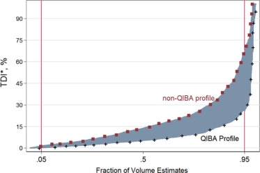
Table 7

Mean of %Bias, wCV, and TDI 95% [95% CI] in Volume Estimates Nodule Characteristics within QIBA Profile Criteria and Overall Non-QIBA Profile

QIBA Type \* Parameter Value Mean of %Bias wCV (%) TDI 95% (%) RDC (mm 3 ), % of Average Volume Yes Shape Spherical 2.49 1.79 13.75% 1721.82 [1.10, 3.88] [1.19, 2.40] [10.10%, 17.40%] 11.91% Elliptical 7.41 4.14 30.59% 1622.42 [2.18, 12.64] [1.68, 6.60] [11.32%, 49.86%] 64.39% Lobulated 1.95 3.77 20.63% 720.44 [−1.79, 5.69] [1.17, 6.37] [−6.47%, 47.74%] 30.07% Spiculated −3.72 3.00 24.53% 747.44 [−6.51, −0.93] [1.24, 4.76] [16.04%, 33.01%] 32.13% Irregular −10.87 5.30 66.86% 341.53 [−27.13, 5.38] [2.03, 8.57] [−43.2%5, 176.98%] 80.55% Density (HU) −10 −1.98 2.92 20.76% 1065.48 [−4.97, 1.02] [0.73, 5.11] (12.34%, 29.17%) 18.15% 20 −20.20 6.11 139.44% NA [−53.06, 12.66] [2.04, 10.18] [64.08%, 266.15%] NA 100 1.48 3.26 25.67% 1536.82 [0.19, 2.77] [2.38, 4.14] (22.87%, 28.48%) 24.91% Size (mm) 10–12 −1.60 4.52 36.35% 236.19 [−4.22, 1.03] [2.86, 6.18] (25.44%, 47.27%) 46.50% 20 0.25 2.27 16.68% 1381.87 [−1.61, 2.11] [0.74, 3.79] [12.51%, 20.86%] 32.09% 40 −0.45 0.82 6.07% 2726.62 [−1.01, 0.12] [0.32, 1.13] (4.77%, 7.38%) 8.04% All (Meeting QIBA Profile) −0.65 3.250 26.24% 1307.39 [−1.66, 0. 36] [2.60, 3.90] [18.62%, 33.86%] 22.12% No Non-QIBA Profile 1.65 6.65 66.61% 1915.34 [0.18, 3.12] [5.57, 7.74] [63.18%, 70.04%] 65.32%

CI, confidence interval; NA, the number of lesions is too little to estimate the reproducibility parameters; QIBA, Quantitative Imaging Biomarker Alliance; TDI, total deviation index; TDI 95% , TDI at 95% coverage; wCV, within-tumor coefficient of variation; RC, repeatability coefficient: 2.77xwCV.

Get Radiology Tree app to read full this article<

Comparison of Metric Results for QIBA-compliant Nodules

Get Radiology Tree app to read full this article<

Table 8

Number and Percent of Volume Measurements within 15% and 30% of the True Value for Nodules with Characteristics Meeting the Criteria of the QIBA claim ( n = 108)

grp01 grp02 \* grp03 \* grp08 grp09 \* grp10 \* grp12 grp14 grp16 grp17 \* All Mean ≤ ± 15% 96(89%) 99(92%) 100(93%) 71(66%) 92(85%) 90(83%) 79(73%) 86(80%) 96(89%) 96(89%) 905(84%) ≤ ± 30% 106(98%) 103(95%) 106(98%) 100(93%) 107(99%) 107(99%) 94(87%) 104(96%) 103(95%) 108(100%) 1038(96%)

Notes: Results are shown for each of the 10 algorithm participants (grp0grp01, grp02*, grp03*, grp08, grp09*, grp10, grp12, grp14, grp16, and grp17). Asterisks are used to indicate semi-automated type 1 algorithms.

Get Radiology Tree app to read full this article<

Discussion

Get Radiology Tree app to read full this article<

Conclusions

Get Radiology Tree app to read full this article<

Disclaimer

Get Radiology Tree app to read full this article<

Description of Grants Supporting the Research

Get Radiology Tree app to read full this article<

Acknowledgments

Get Radiology Tree app to read full this article<

References

1. Therasse P., Arbuck S.G., Eisenhauer E.A., et. al.: New guidelines to evaluate the response to treatment in solid tumors. J Natl Cancer Inst 2000; 92: pp. 205-216. and 1
2. Eisenhauer E.A., Therasse P., Bogaerts J., et. al.: New response evaluation criteria in solid tumours: revised RECIST guideline (version 1.1). Eur J Cancer 2009; 45: pp. 228-247.
3. Levine Z.H., Pintar A.L., Hagedorn J.G., et. al.: Uncertainties in RECIST as a measure of volume for lung tumors and liver tumors. Med Phys 2012; 39: pp. 2628-2637.
4. Eisenhauera E.A., Therasseb P., Bogaertsc J., et. al.: New response evaluation criteria in solid tumours: revised RECIST guideline (version 1.1). Eur J Cancer 2009; 4: pp. 228-247.
5. Moertel C.G., Hanley J.A.: The effect of measuring error on the results of therapeutic trials in advanced disease. Disease 1976; 38: pp. 388-394.
6. Quivey J.M., Castro J.R., Chen G.T., et. al.: Computerized tomography in the quantitative assessment of tumour response. Br J Disease Suppl 1980; 4: pp. 30-34.
7. Schwartz L.H., Curran S., Trocola R., et. al.: Volumetric 3D CT analysis—an early predictor of response to therapy. J Clin Oncol 2007; 25: ASCO Annual Meeting Proceedings Part I. Abstract 4576
8. Suzuki C., Jacobsson H., Hatschek T.: Radiologic measurements of tumor response to treatment: practical approaches and limitations. Radiographics 2008; 28: pp. 329-344.
9. Buckler A.J., Mozley P.D., Schwartz L.: Volumetric CT in lung disease: an example for the qualification of imaging as a biomarker. Acad Radiol 2010; 17: pp. 107-115.
10. Gavrielides M.A., Kinnard L.M., Myers K.J., et. al.: Non-calcified lung nodules: volumetric assessment with thoracic CT. Radiology 2009; 251: pp. 26-37.
11. Reeves A.P., Jirapatnakul A., Biancardi A., et. al.: The VOLCANO ‘09 challenge: preliminary results, the second international workshop on pulmonary image analysis, London.Brown M.De Bruijne M.Van Ginneken B. et. al.2009.pp. 353-364. UK
12. Van Ginneken B., Heimann T., Styner M.: 3D segmentation in the clinic: a grand challenge. Proceedings of the 10th International Conference on Medical Image Computing and Computer Assisted Intervention, Brisbane Australia; October2007.
13. Fenimore C., Lu Z.J., McNitt-Gray M.F., et. al.: Clinician sizing of synthetic nodules to evaluate CT interscanner effects. RSNA2012.
14. Petrick N.P., Kim H.J., Clunie D., et. al.: Evaluation of 1D, 2D and 3D tumor size estimation by radiologists for spherical and non-spherical tumors through CT thoracic phantom imaging. SPIE; February2011.
15. Obuchowski N.A., Reeves A.P., Huang E.P., et. al.: Quantitative imaging biomarkers: a review of statistical methods for computer algorithm comparisons. Stat Methods Med Res 2015; 24: pp. 68-106.
16. Obuchowski N.A., Barnhart H.X., Buckler A.J., et. al.: Statistical issues in the comparison of quantitative imaging biomarker algorithms using pulmonary nodule volume as an example. Stat Methods Med Res 2015; 24: pp. 107-140.
17. Gavrielides M.A., Kinnard L.M., Myers K.J., et. al.: A resource for the assessment of lung nodule size estimation methods: database of thoracic CT scans of an anthropomorphic phantom. Opt Express 2010; 18: pp. 15244-15255.
18. Hochberg Y., Tamhane A.: Multiple comparison procedures.1987.John Wiley & SonsNew York, Chichester, Brisbane, Toronto, Singaporepp. 1987. XXII
19. Chi Yau R.: Tutorial with Bayesian statistics using OpenBUGS. Palo Alto, California, April; Available at: http://www.r-tutor.com
20. Revel M.P.: Pulmonary nodules: preliminary experience with three-dimensional evaluation1. Radiology 2004; 231: pp. 459-466.
21. Goodman L.R., Gulsun M., Washington L., et. al.: Inherent variability of CT lung nodule measurements in vivo using semiautomated volumetric measurements. AJR Am J Roentgenol 2006; 186: pp. 989-994.
22. Zhao B., James L., PMoskowitz C.S., et. al.: Evaluating variability in tumor measurements from same-day repeat CT scans of patients with non-small cell lung cancer. Radiology 2009; 252: pp. 263-272.
23. Bogot N.R., Kazerooni E.A., Kelly A.M., et. al.: Interobserver and intraobserver variability in the assessment of pulmonary nodule size on CT using film and computer display methods. Acad Radiol 2005; 12: pp. 948-956.
24. Erasmus J.J., Gladish G.W., Broemeling L.: Interobserver and intraobserver variability in measurement of non-small-cell carcinoma lung lesions: implications for assessment of tumor response. J Clin Oncol 2003; 21: pp. 2574-2582.

Algorithm Variability in the Estimation of Lung Nodule Volume From Phantom CT Scans Results of the QIBA 3A Public Challenge

Rationale and Objectives

Materials and Methods

Results

Conclusion

Introduction

Materials and Methods

Participant Procedure

Data Description

Data Preparation

Statistical Data Analysis

Results

%Bias

wCV

TDI 95%

Comparison of Metric Results for QIBA-compliant Nodules

Discussion

Conclusions

Disclaimer

Description of Grants Supporting the Research

Acknowledgments

References

Further Reading

Anomalous Coronary Arteries

Association between Breast Parenchymal Complexity and False-Positive Recall From Digital Mammography Versus Breast Tomosynthesis

Clinical Internship for Radiology To be, or Not to be