
Rationale and Objectives
The estimation of the area under the receiver operating characteristic (ROC) curve (AUC) often relies on the assumption that the truly positive population tends to have higher marker results than the truly negative population. The authors propose a discriminatory measure to relax such an assumption and apply the measure to identify the appropriate set of markers for combination.
Materials and Methods
The proposed measure is based on the maximum of the AUC and 1-AUC. The existing methods are applied to estimate the measure. The subset of markers is selected using a combination method that maximizes a function of the proposed discriminatory score with the number of markers as a penalty in the function.
Results
The properties of the estimators for the proposed measure were studied through large-scale simulation studies. The application was illustrated through a real example to identify the set of markers to combine.
Conclusion
Simulation results showed excellent small-sample performance of the estimators for the proposed measure. The application in the example yielded a reasonable subset of markers for combination.
The receiver operating characteristic (ROC) curves have become an important tool for evaluating the accuracy of diagnostic markers and have been found useful in many areas of scientific research such as diagnostic imaging , signal detection, and biometric identification . The ROC curve of a marker is obtained by plotting, over all possible values of the marker results, the true-positive rate (or sensitivity), the probability that the marker correctly identifies a truly positive subject, versus the false-positive rate (or 1 − specificity), the probability that the marker incorrectly identifies a truly negative subject.
The area under the ROC curve (AUC) has been recognized as an important measure of the accuracy of the marker . An AUC value close to 1 indicates high discriminatory power of a diagnostic marker, and a value of 0.5 suggests that a marker has a diagnostic ability no better than tossing a fair coin. Many authors developed methods to estimate the AUC, among which some are nonparametric , some are parametric , and some are semiparametric .
Get Radiology Tree app to read full this article<
Get Radiology Tree app to read full this article<
Get Radiology Tree app to read full this article<
Materials and methods
Brief Review of ROC Curves
Get Radiology Tree app to read full this article<
Get Radiology Tree app to read full this article<
Get Radiology Tree app to read full this article<
Get Radiology Tree app to read full this article<
Discriminatory Measure of Markers
Get Radiology Tree app to read full this article<
Selection of a Group of Markers with High Discriminatory Power: An Additive Procedure
Get Radiology Tree app to read full this article<
Get Radiology Tree app to read full this article<
Get Radiology Tree app to read full this article<
Get Radiology Tree app to read full this article<
Get Radiology Tree app to read full this article<
Description of the Simulation Studies
Get Radiology Tree app to read full this article<
Get Radiology Tree app to read full this article<
Table 1
Additive Procedure for Combining Markers: An Example
IGFII IGFBP3 IGF1 DHEAiˆk i
ˆ
k 0.7659 0.7372 0.6779 0.5189
DHEA, dehydroepiandrosterone; IGF, insulin-like growth factor; IGFBP, IGF binding protein.
Table 2
Monte Carlo Bias and RMSE (Normal Data, nsim = 10,000)
Configuration
(μN,μD,σN,σD) (
μ
N
,
μ
D
,
σ
N
,
σ
D
) Estimator Sample Sizes ( n 1 , n 2 ) (10,10) (20,30) (50,50) (50,100) Bias (RMSE) Bias (RMSE) Bias (RMSE) Bias (RMSE) (0, 0, 1, 1) P 0.100 (0.126) 0.065 (0.081) 0.045 (0.057) 0.039 (0.049) NP 0.106 (0.132) 0.067 (0.084) 0.047 (0.058) 0.040 (0.050) (0, 0, 2, 5) P 0.103 (0.130) 0.060 (0.076) 0.046 (0.057) 0.034 (0.043) NP 0.111 (0.139) 0.065 (0.082) 0.050 (0.062) 0.036 (0.046) (0, 0.5, 1, 1) P 0.016 (0.099) 0.004 (0.073) −0.001 (0.053) 0.000 (0.047) NP 0.020 (0.103) 0.005 (0.075) −0.001 (0.054) 0.001 (0.048) (0, 0.5, 2, 5) P 0.071 (0.107) 0.031 (0.059) 0.017 (0.043) 0.010 (0.034) NP 0.080 (0.116) 0.036 (0.064) 0.020 (0.046) 0.012 (0.036) (0, 1, 1, 1) P −0.002 (0.100) −0.002 (0.067) −0.001 (0.047) 0.000 (0.040) NP 0.002 (0.105) 0.002 (0.069) −0.001 (0.047) 0.001 (0.041) (0, 1, 2, 5) P 0.044 (0.098) 0.013 (0.061) 0.005 (0.049) 0.002 (0.040) NP 0.052 (0.105) 0.016 (0.064) 0.007 (0.052) 0.003 (0.042)
AUC, area under the curve; NP, nonparametric AUC estimator; nsim, number of simulations; P, parametric (normal-based) AUC estimator; RMSE, root mean square error.
Table 3
Monte Carlo Bias and RMSE (Lognormal Data, nsim = 10,000)
Configuration
(μN,μD,σN,σD) (
μ
N
,
μ
D
,
σ
N
,
σ
D
) ∗ Estimator Sample Sizes ( n 1 , n 2 ) (10,10) (20,30) (50,50) (50,100) Bias (RMSE) Bias (RMSE) Bias (RMSE) Bias (RMSE) (0, 0, 1, 1) P 0.104 (0.130) 0.066 (0.083) 0.046 (0.057) 0.040 (0.049) NP 0.106 (0.132) 0.067 (0.084) 0.047 (0.058) 0.040 (0.050) (0, 0, 2, 5) P 0.110 (0.138) 0.065 (0.081) 0.047 (0.059) 0.035 (0.044) NP 0.111 (0.139) 0.066 (0.083) 0.048 (0.060) 0.037 (0.046) (0, 0.5, 1, 1) P 0.018 (0.101) 0.003 (0.073) 0.001 (0.054) 0.001 (0.047) NP 0.019 (0.102) 0.003 (0.074) 0.002 (0.055) 0.001 (0.047) (0, 0.5, 2, 5) P 0.078 (0.115) 0.034 (0.063) 0.019 (0.045) 0.010 (0.035) NP 0.078 (0.116) 0.035 (0.064) 0.020 (0.046) 0.011 (0.036) (0, 1, 1, 1) P 0.001 (0.100) −0.001 (0.067) 0.000 (0.047) 0.000 (0.041) NP 0.002 (0.105) −0.001 (0.069) 0.001 (0.048) 0.000 (0.041) (0, 1, 2, 5) P 0.051 (0.103) 0.015 (0.063) 0.006 (0.051) 0.002 (0.041) NP 0.052 (0.105) 0.016 (0.064) 0.007 (0.052) 0.002 (0.042)
AUC, area under the curve; NP, nonparametric AUC estimator; nsim, number of simulations; P, parametric (normal-based) AUC estimator; RMSE, root mean square error.
Get Radiology Tree app to read full this article<
Table 4
Monte Carlo Bias and RMSE (Normal Mixture Data, nsim = 10,000)
Configuration
(μN,μD,σN,σD) (
μ
N
,
μ
D
,
σ
N
,
σ
D
) Estimator Sample Sizes ( n 1 , n 2 ) (10,10) (20,30) (50,50) (50,100) Bias (RMSE) Bias (RMSE) Bias (RMSE) Bias (RMSE) (0, 0, 1, 1) P 0.104 (0.130) 0.066 (0.083) 0.046 (0.057) 0.039 (0.049) NP 0.105 (0.132) 0.067 (0.084) 0.047 (0.058) 0.040 (0.050) (0, 0, 2, 5) P 0.107 (0.133) 0.063 (0.078) 0.047 (0.058) 0.035 (0.044) NP 0.111 (0.139) 0.066 (0.082) 0.049 (0.062) 0.037 (0.046) (0, 0.5, 1, 1) P 0.016 (0.098) 0.005 (0.073) 0.002 (0.054) 0.000 (0.047) NP 0.018 (0.101) 0.006 (0.074) 0.004 (0.055) 0.000 (0.047) (0, 0.5, 2, 5) P 0.068 (0.106) 0.026 (0.056) 0.015 (0.044) 0.006 (0.032) NP 0.078 (0.116) 0.034 (0.063) 0.022 (0.049) 0.010 (0.036) (0, 1, 1, 1) P −0.003 (0.099) −0.001 (0.067) −0.001 (0.047) 0.000 (0.040) NP −0.002 (0.105) 0.002 (0.069) 0.001 (0.048) 0.001 (0.041) (0, 1, 2, 5) P 0.038 (0.094) 0.003 (0.058) 0.001 (0.044) 0.000 (0.039) NP 0.048 (0.100) 0.015 (0.064) 0.008 (0.053) 0.002 (0.043)
AUC, area under the curve; NP, nonparametric AUC estimator; nsim, number of simulations; P, parametric (normal-based) AUC estimator; RMSE, root mean square error.
0.8N(μi,32√4σi)+0.2N(μi,2√2σi) 0.8
N
(
μ
i
,
3
2
4
σ
i
)
+
0.2
N
(
μ
i
,
2
2
σ
i
) , i=N,D i
=
N
,
D .
Table 5
Monte Carlo Bias and RMSE (Lognormal Mixture Data, nsim = 10,000)
Configuration
(μN,μD,σN,σD) (
μ
N
,
μ
D
,
σ
N
,
σ
D
) ∗ Estimator Sample Sizes ( n 1 , n 2 ) (10,10) (20,30) (50,50) (50,100) Bias (RMSE) Bias (RMSE) Bias (RMSE) Bias (RMSE) (0, 0, 1, 1) P 0.103 (0.129) 0.068 (0.083) 0.045 (0.057) 0.039 (0.049) NP 0.104 (0.131) 0.069 (0.085) 0.047 (0.059) 0.040 (0.050) (0, 0, 2, 5) P 0.114 (0.141) 0.074 (0.091) 0.058 (0.072) 0.047 (0.058) NP 0.106 (0.133) 0.065 (0.082) 0.051 (0.063) 0.037 (0.046) (0, 0.5, 1, 1) P 0.019 (0.100) 0.003 (0.075) 0.002 (0.053) −0.001 (0.047) NP 0.018 (0.100) 0.003 (0.076) 0.003 (0.054) −0.000 (0.047) (0, 0.5, 2, 5) P 0.085 (0.121) 0.051 (0.080) 0.041 (0.066) 0.035 (0.056) NP 0.073 (0.110) 0.034 (0.064) 0.022 (0.050) 0.010 (0.037) (0, 1, 1, 1) P 0.002 (0.101) 0.002 (0.068) 0.001 (0.047) −0.001 (0.041) NP 0.003 (0.105) 0.002 (0.069) 0.002 (0.047) −0.001 (0.041) (0, 1, 2, 5) P 0.064 (0.112) 0.040 (0.080) 0.035 (0.067) 0.033 (0.057) NP 0.048 (0.100) 0.016 (0.065) 0.009 (0.053) 0.002 (0.043)
AUC, area under the curve; NP, nonparametric AUC estimator; nsim, number of simulations; P, parametric (normal-based) AUC estimator; RMSE, root mean square error.
Get Radiology Tree app to read full this article<
Get Radiology Tree app to read full this article<
Description of Real Data Analysis
Get Radiology Tree app to read full this article<
Results
Get Radiology Tree app to read full this article<
Get Radiology Tree app to read full this article<
Get Radiology Tree app to read full this article<
Get Radiology Tree app to read full this article<
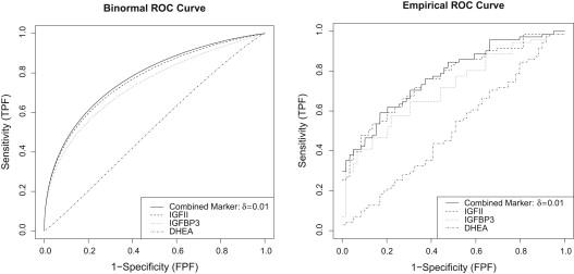
0.0255×IGFII+0.5196×IGFBP3−0.2576×DHEA, 0.0255
×
IGFII
+
0.5196
×
IGFBP
3
−
0.2576
×
DHEA,
and estimated iˆk=0.7768 i
ˆ
k
=
0.7768 . To put more penalty on the number of markers, we set δ=0.05 δ
=
0.05 and only the first marker IGFII is selected with estimated iˆk=0.7659 i
ˆ
k
=
0.7659 . Alternatively, less penalty can be considered so that δ=0.005 δ
=
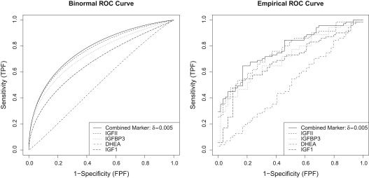
0.005 , and we include all markers in the selection. The resulting combination of all markers {IGFII, IGFBP3, DHEA, IGF1} is
0.0248×IGFII+0.4514×IGFBP3−0.2681×DHEA+0.0069×IGF1 0.0248
×
IGFII
+
0.4514
×
IGFBP
3
−
0.2681
×
DHEA
+
0.0069
×
IGF
1
with estimated iˆk=0.7777 i
ˆ
k
=
0.7777 .
Get Radiology Tree app to read full this article<
Get Radiology Tree app to read full this article<
Get Radiology Tree app to read full this article<
Discussion
Get Radiology Tree app to read full this article<
Get Radiology Tree app to read full this article<
Get Radiology Tree app to read full this article<
Get Radiology Tree app to read full this article<
AIC=−2ln(L(θ1,…,θp))+2p,BIC=−2ln(L(θ1,…,θp))+pln(n), A
I
C
=
−
2
ln
(
L
(
θ
1
,
…
,
θ
p
)
)
+
2
p
,
B
I
C
=
−
2
ln
(
L
(
θ
1
,
…
,
θ
p
)
)
+
p
ln
(
n
)
,
where L(θ1,…,θp) L
(
θ
1
,
…
,
θ
p
) is the likelihood function of p parameters θ1 θ
1 , …, θp θ
p , and n is the number of observations. Suppose that observations from multiple markers follow a multivariate normal distribution. In the AIC and BIC criteria, the parameters θ1,…,θp θ
1
,
…
,
θ
p are means, variances and correlation coefficients to be estimated, and the likelihood function L(θ1,…,θp) L
(
θ
1
,
…
,
θ
p
) are derived by multiplying the density distributions. For the two-sample case that is considered in the ROC literature, we can consider the AIC and BIC in the following fashion:
AIC*=−2ln(L1(θ1,…,θp)L2(θ*1,…,θ*p))+2×2p,BIC*=−2ln(L1(θ1,…,θp)L2(θ*1,…,θ*p))+2pln(m+n). A
I
C
*
=
−
2
ln
(
L
1
(
θ
1
,
…
,
θ
p
)
L
2
(
θ
1
*
,
…
,
θ
p
*
)
)
+
2
×
2
p
,
B
I
C
*
=
−
2
ln
(
L
1
(
θ
1
,
…
,
θ
p
)
L
2
(
θ
1
*
,
…
,
θ
p
*
)
)
+
2
p
ln
(
m
+
n
)
.
Get Radiology Tree app to read full this article<
Get Radiology Tree app to read full this article<
Acknowledgments
Get Radiology Tree app to read full this article<
Appendix
Property of iˆk i ˆ k and Some Proof
Get Radiology Tree app to read full this article<
iˆk=max{1mn∑mi=1∑nj=1I(Xki>Ykj),1mn∑mi=1∑nj=1I(Xki<Ykj)}. i
ˆ
k
=
max
{
1
m
n
∑
i
=
1
m
∑
j
=
1
n
I
(
X
k
i
Y
k
j
)
,
1
m
n
∑
i
=
1
m
∑
j
=
1
n
I
(
X
k
i
<
Y
k
j
)
}
.
and β=σN/σD β
=
σ
N
/
σ
D .
Get Radiology Tree app to read full this article<
Get Radiology Tree app to read full this article<
ik=Φ(|μkD−μkN|σ2kN+σ2kD√). i
k
=
Φ
(
|
μ
k
D
−
μ
k
N
|
σ
k
N
2
+
σ
k
D
2
)
.
and its estimator iˆk i
ˆ
k is obtained by substituting the mean parameters by the sample means, and the variance parameters by the sample variances. We can show that the estimator is approximately normally distributed with mean zero. The proof is available upon request from the authors.
Get Radiology Tree app to read full this article<
Multivariate Normal Distributions
Get Radiology Tree app to read full this article<
The Discriminatory Score Based on the Optimal Linear Combination
Get Radiology Tree app to read full this article<
λ∗=(ΣX+ΣY)−1(μX−μY). λ
∗
=
(
Σ
X
+
Σ
Y
)
−
1
(
μ
X
−
μ
Y
)
.
Get Radiology Tree app to read full this article<
Get Radiology Tree app to read full this article<
iK=Φ((μX−μY)(ΣY+ΣY)−1(μX−μY)−−−−−−−−−−−−−−−−−−−−−−−−−−−√). i
K
=
Φ
(
(
μ
X
−
μ
Y
)
(
Σ
Y
+
Σ
Y
)
−
1
(
μ
X
−
μ
Y
)
)
.
Get Radiology Tree app to read full this article<
References
1. Swets J.: Form of empirical ROCs in discrimination and diagnostic tasks: implications for theory and measurement of performance. Psychological Bulletin 1986; 99: pp. 181-198.
2. Metz C.E.: Basic principles of ROC analysis. Semin Nucl Med 1978; 8: pp. 283-298. URL http://www.sciencedirect.com/science/article/pii/S0001299878800142
3. Alemayehu D., Zou K.H.: Applications of ROC analysis in medical research: recent developments and future directions. Acad Radiol 2012; 19: pp. 1457-1464.
4. Eng J.: Sampling the latest work in receiver operating characteristic analysis: What does it mean?. Acad Radiol 2012; 19: pp. 1449-1451.
5. Hanley J., McNeil B.: A method of comparing the areas under (ROC) curves derived from same cases. Radiology 1983; 148: pp. 839-843.
6. Pesce L., Metz C., Berbaum K.: On the convexity of roc curves estimated from radiological test results. Acad Radiol 2010; 17: pp. 960-968.
7. Bolle R., Connell J., Pankanti S., et. al.: Guide to biometrics.2004.SpringerNew York
8. Hanley J., McNeil B.: The meaning and use of the area under a receiver operating characteristic (ROC) curve. Radiology 1982; 143: pp. 29-36.
9. Wieand S., Gail M.H., James B.R., et. al.: A family of nonparametric statistics for comparing diagnostic markers with paired or unpaired data. Biometrika 1989; 76: pp. 585-592.
10. DeLong E.R., DeLong D., Clarke-Pearson D.: Comparing the areas under two or more correlated receiver operating characteristic curves: A nonparametric approach. Biometrics 1988; 44: pp. 837-845.
11. Reiser B., Guttman I.: Statistical-inference for pr(y-less-than-x) - the normal case. Technometrics 1986; 28: pp. 253-257.
12. Metz C.E., Herman B.A., Shen J.-H.: Maximum likelihood estimation of receiver operating characteristic (roc) curves from continuously-distributed data. Stat Med 1998; 17: pp. 1033-1053. URL http://dx.doi.org/10.1002/(SICI)1097-0258(19980515)17:9<1033::AID-SIM784>3.0.CO;2-Z
13. Dorfman D.D., Alf E.: Maximum likelihood estimation of parameters of signal detection theory and determination of confidence intervals-rating method data. J Math Psychol 1969; 6: pp. 487-496.
14. Zou K., Hall W., Shapiro D.: Smooth non-parametric receiver operating characteristic (ROC) curves for continuous diagnostic tests. Stat Med 1997; 16: pp. 2143-2156.
15. Pepe M.S.: Three approaches to regression analysis of receiver operating characteristic curves for continuous test results. Biometrics 1998; 54: pp. 124-135.
16. Pesce L., Horsch K., Drukker K., et. al.: Semiparametric estimation of the relationship between roc operating points and the test-result scale: application to the proper binormal model. Acad Radiol 2011; 18: pp. 1537-1548.
17. Tang L.L., Zhou X.-H.: A semiparametric separation curve approach for comparing correlated roc data from multiple markers. J Comput Graphical Stat 2012; 21: pp. 662-676. URL http://www.tandfonline.com/doi/abs/10.1080/10618600.2012.663303
18. Zhou X.H., Obuchowski N.A., McClish D.K.: Statistical methods in diagnostic medicine.2002.WileyNew York
19. Pepe M.S.: The statistical evaluation of medical tests for classification and prediction.2003.Oxford University PressNew York
20. Zou K.H., Liu A., Bandos A.L., et. al.: Statistical evaluation of diagnostic performance: topics in ROC analysis.2011.Chapman & HallCRC
21. Bamber D.: The area above the ordinal dominance graph and the area below the receiver operating characteristic graph. J Math Psychol 1975; 12: pp. 387-415.
22. Metz C.E., Wang P.-L., Kronman H.: A new approach for testing the significance of differences between roc curves measured from correlated data.Deconinck F.Information processing in medical imaging: proceedings of the eighth conference.1984.Martinus NijhoffThe Hague:
23. Zou K., Warfield S., Fielding J., et. al.: Statistical validation based on parametric receiver operating characteristic analysis of continuous classification data. Acad Radiol 2003; 10: pp. 1359-1368.
24. Zou K.H., Warfield S.K., Bharatha A., et. al.: Statistical validation of image segmentation quality based on a spatial overlap index1: scientific reports. Acad Radiol 2004; 11: pp. 178-189. URL http://www.sciencedirect.com/science/article/pii/S1076633203006718
25. Kramar A., Faraggi D., Ychou M., et. al.: The generalized ROC criterion for the evaluation of several tumor markers. Revue d’Epidemiologie ei de Sante Publique 1999; 47: pp. 217-226.
26. Schisterman E. Lipid peroxidation and antioxidant biomarkers and biomarker disease. Doctoral dissertation, State University of New York at Buffalo; 1999.
27. Su J.Q., Liu J.S.: Linear combinations of multiple diagnostic markers. J Am Stat Assoc 1993; 88: pp. 1350-1355. URL http://www.jstor.org/stable/2291276
28. Mills J.L., Hediger M.L., Molloy C.A., et. al.: Elevated levels of growth-related hormones in autism and autism spectrum disorder. Clin Endocrinol 2007; 67: pp. 230-237. URL http://dx.doi.org/10.1111/j.1365-2265.2007.02868.x
29. Liu A., Li Q., Liu C., et. al.: A rank-based test for comparison of multidimensional outcomes. J Am Stat Assoc 2010; 105: pp. 578-587. URL http://amstat.tandfonline.com/doi/abs/10.1198/jasa.2010.ap09114
30. Hillis S., Metz C.: An analytic expression for the binormal partial area under the roc curve. Acad Radiol 2012; 19: pp. 1491-1498.
31. Bozdogan H.: Model selection and akaike’s information criterion (AIC): the general theory and its analytical extensions. Psychometrika 1987; 52: pp. 345-370.
32. Schwarz G.: Estimating the dimension of a model. Ann Stat 1978; 6: pp. 461-464.
33. Demler O., Pencina M., et. al.: Misuse of Delong test to compare AUCs for nested models. Stat Med 2012; 31: pp. 2577-2587.
34. Vickers A., Cronin A., Begg C.: One statistical test is sufficient for assessing new predictive markers. BMC Med Res Methodol 2011; 11: pp. 13.