An Anthropomorphic Breast Model for Breast Imaging Simulation and Optimization

Rationale and Objectives

Optimization studies for x-ray−based breast imaging systems using computer simulation can greatly benefit from a phantom capable of modeling varying anatomical variability across different patients. This study aimed to develop a three-dimensional phantom model with realistic and randomizable anatomical features.

Materials and Methods

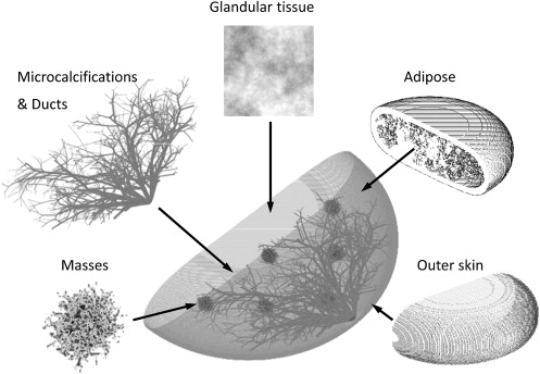
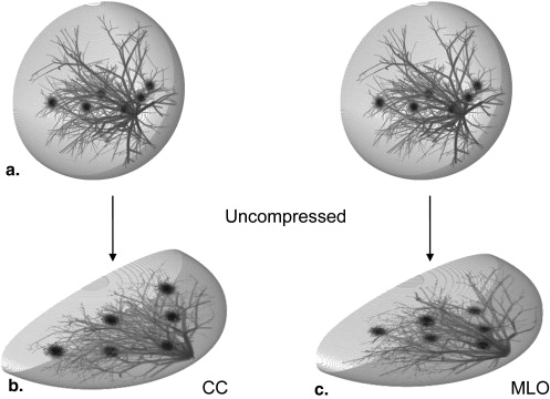
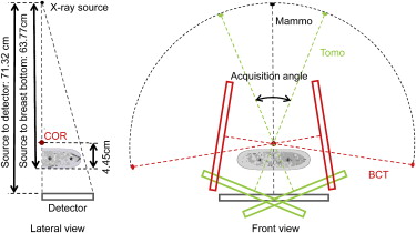
A voxelized breast model was developed consisting of an outer layer of skin and subcutaneous fat, a mixture of glandular and adipose, stochastically generated ductal trees, masses, and microcalcifications. Randomized realization of the breast morphology provided a range of patient models. Compression models were included to represent the breast under various compression levels along different orientations. A Monte Carlo (MC) simulation code was adapted to simulate x-ray based imaging systems for the breast phantom. Simulated projections of the phantom at different angles were generated and reconstructed with iterative methods, simulating mammography, breast tomosynthesis, and computed tomography (CT) systems. Phantom dose maps were further generated for dosimetric evaluation.

Results

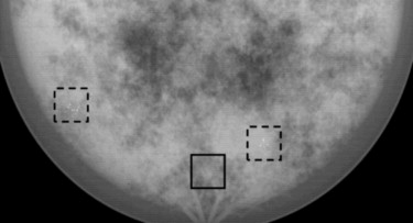
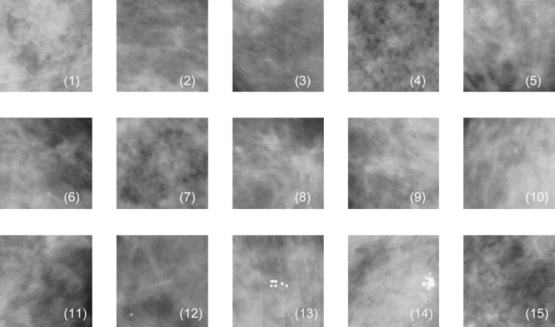
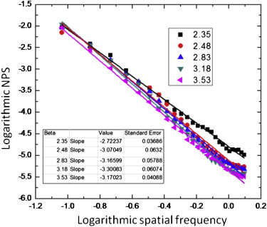
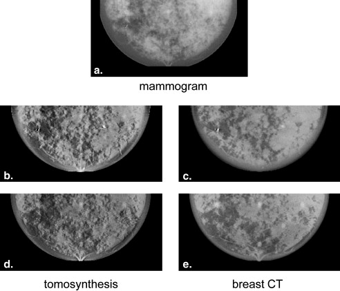
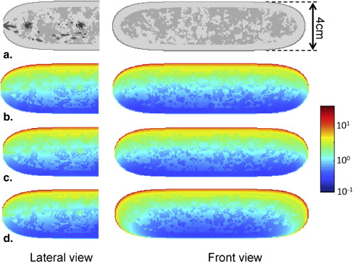
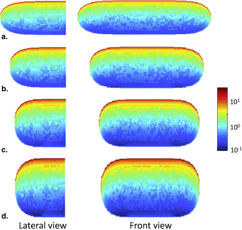
Region of interest comparisons of simulated and real mammograms showed strong similarities in terms of appearance and features. Noise-power spectra of simulated mammographic images demonstrated that the phantom provided target properties for anatomical backgrounds. Reconstructed tomosynthesis and CT images and dose maps provided corresponding data from a single breast enabling optimization studies. Dosimetry result provided insight into the dose distribution difference between modalities and compression levels.

Conclusion

The anthropomorphic breast phantom, combined with the MC simulation platform, generated a realistic model for a breast imaging system. The developed platform is expected to provide a versatile and powerful framework for optimizing volumetric breast imaging systems.

Breast imaging performance is highly affected by the spatial heterogeneity of the breast structure . Furthermore, breast density varies substantially across patients of different ages . As a result, optimizing breast imaging systems across a variety of cases requires the capability of modeling the heterogeneity and variability across patients. In recent years, a number of anthropomorphic breast models have been developed for breast-related research, including physical and computerized phantoms . Physical phantoms were employed for empirical performance measurements , whereas computerized phantoms were voxelized and embedded into computerized simulations . Computerized phantoms have shown advantages in optimization research because of their low cost, ability to imitate subtle tissue structures, and ability to represent varying physical properties. These phantoms are generally characterized into two categories: those based on data from computed tomography (CT) or magnetic resonance imaging (MRI) scans , and those defined by analytical descriptions of human anatomy . Phantoms based on CT or MRI data are highly realistic, because they are built from patient data; however, they are inherently limited by the employed scanning technique (eg, finite resolution, noise pattern, artifact). Furthermore, these phantoms are not representative of the whole population, because each phantom is built from one specific patient. In contrast, phantoms based on mathematical methods are not restricted by the imaging technique. While being not as realistic, they offer a larger flexibility of parameter, enabling breast models representative of large segments of the population. Furthermore, recent studies to improve on the realism of these phantoms have included advanced mathematical concepts such as fractal structure and self-similar structure implemented to model realistic breast structures .

Based on prior research, this work focuses on developing a mathematical breast phantom with compression models, which includes skin, adipose tissue, glandular tissue, ducts, microcalcifications, and masses . The phantom presented here improves on prior work in several ways with more realistic skin boundary definition, more accurate anatomical background structure, improved ductal connections and distribution, increased number of growing features in the stochastic mass definition, added microcalcifications, and the development of a deformation algorithm that compresses the breast along various orientations into various thicknesses objects. This project further includes dedicated Monte Carlo (MC) projection simulation and iterative image reconstruction software for simulating and optimizing breast imaging modalities.

Materials and methods

Breast Phantom Construction

Get Radiology Tree app to read full this article<

Skin

Get Radiology Tree app to read full this article<

Background Texture

Get Radiology Tree app to read full this article<

P(f)=1fβ, P

(

)

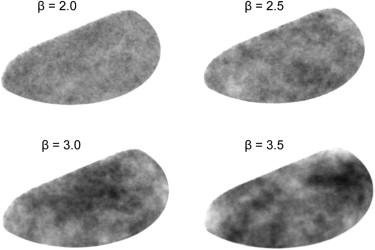
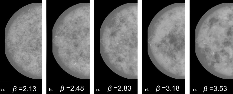
where f denotes spatial frequency and the β factor denotes the Hausdorff dimension of a fractal structure . Previous research suggested that mammograms possess a mean β value of 2.83 with a standard deviation of 0.35 , and that the β value in a two-dimensional mammographic projection corresponds to the β value in the three-dimensional (3D) volume . Thus, the 3D texture in this work employed a β values randomly selected between 2.13 and 3.53 (ie, β =2.83 ± 2*0.35).

Get Radiology Tree app to read full this article<

H(u,v,w)=⎧⎩⎨⎪⎪01(u2+v2+w2√)β2u=v=w=0otherwise, H

(

)

{

(

)

where (u,v,w)∈[(−U,−V,−W),(U,V,W)], (

)

∈

[

(

−

)

(

)

]

, and U, V, and W correspond to the Nyquist frequencies in the orthogonal direction (ie, 12Δx,12Δy,12Δz, 1

, with Δx,Δy,Δz Δ

z characterizing the voxel size in three dimensions). The filtered volume representing the designed inverse power law distribution was converted to spatial domain by inverse Fourier transform, and thresholded by assigning each voxel to either a glandular or an adipose tissue value to produce the desired glandular tissue density. This thresholded matrix, however, had glandular and adipose tissue scattered and discontinued within the volume. To better imitate the pattern of background tissues, an additional smoothing process was performed to expand both the glandular and adipose region to be continuous.

Get Radiology Tree app to read full this article<

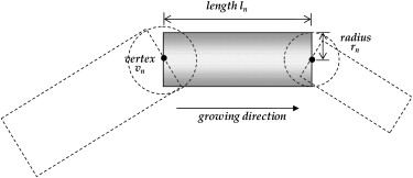
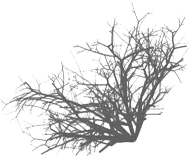
Ductal Network

Get Radiology Tree app to read full this article<

Table 1

Parameters Used in the Ductal System Simulation for a Reasonable Visual Pattern

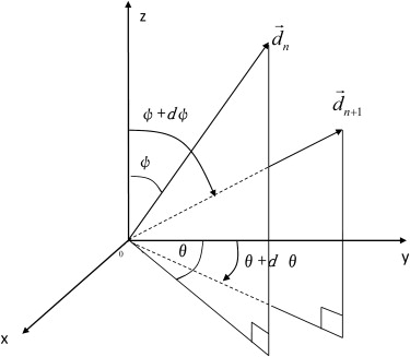
Parameter Symbol Value Radius of level 0r 0 1 mm Length of level 0l 0 5 mm Probability of a smaller progeny_p_ 1 32% Probability of bifurcation_p_ 2 28% Probability of no new progeny_p_ 3 40% Scaling factor between radii_a_ 0.8 Factor between radius and length_b_ 8 Lower limitation of segment length_q_ 1 % 40% Upper limitation of segment length_q_ 2 % 100% Polar angle of the new branch ± (37.5° ± 10°) Azimuthal angle of the new branch_φ_ ± (15° ± 5°)

Get Radiology Tree app to read full this article<

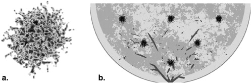
Microcalcification

Get Radiology Tree app to read full this article<

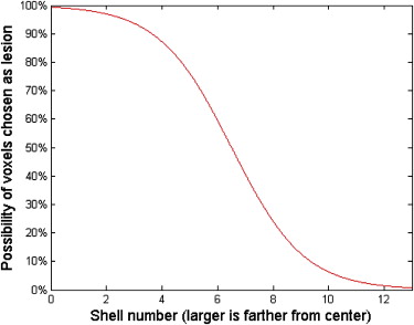
Breast Masses

Get Radiology Tree app to read full this article<

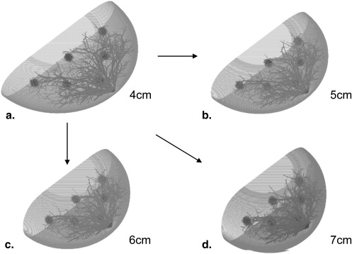
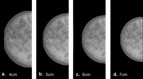
Compression Models

Get Radiology Tree app to read full this article<

(rR)6+(zT/2)2=1,wherer2=x2+y2,y>0. (

)

(

)

where

Get Radiology Tree app to read full this article<

x’=1α√x,y’=1α√y,z’=αz. x

′

Get Radiology Tree app to read full this article<

(xR’)2+(yR’)2+(zR’)2=1,y>0. (

′

)

(

′

)

(

′

)

Get Radiology Tree app to read full this article<

(x’R)2+(y’R)2+(|z’|T/2)2.75=1,y’>0. (

′

)

(

′

)

(

′

)

2.75

′

Get Radiology Tree app to read full this article<

(xR’)2=(x’R)2,(yR’)2=(y’R)2,(zR’)2=(|z’|T/2)2.75. (

′

)

(

′

)

(

′

)

(

′

)

(

′

)

(

′

)

2.75

Get Radiology Tree app to read full this article<

Phantom and System Validation

Get Radiology Tree app to read full this article<

Dosimetric Evaluation

Get Radiology Tree app to read full this article<

D=dϵdm=dϵρdV, D

where dϵ d

ϵ denotes the local deposited energy, dm denotes the mass of the voxel, ρ ρ denotes the density of the material in the voxel, and dV denoted the volume of the voxel. A 3D dose map representing the dose distribution in the breast phantom was generated after calculating the deposited dose in each voxel.

Get Radiology Tree app to read full this article<

Results

Mammographic Simulations

Get Radiology Tree app to read full this article<

β value Validation

Get Radiology Tree app to read full this article<

Volumetric Imaging

Get Radiology Tree app to read full this article<

Dosimetry

Get Radiology Tree app to read full this article<

Discussion

Get Radiology Tree app to read full this article<

References

1. Samei E., Eyler W., Baron L.: Effects of anatomical structure on signal detection. Handbook of Medical Imaging.2000.SPIE PressBellingham, WA
2. Tamimi R.M., Cox D., Kraft P., et. al.: Breast cancer susceptibility loci and mammographic density. Breast Cancer Res 2008; 10: pp. R66.
3. Armstrong K., Eisen A., Weber B.: Assessing the risk of breast cancer. N Engl J Med 2000; 342: pp. 564-571.
4. Caldwell C.B., Yaffe M.J.: Development of an anthropomorphic breast phantom. Med Phys 1990; 17: pp. 273-280.
5. Cinti M.N., Pani R., Garibaldi F., et. al.: Custom breast phantom for an accurate tumor SNR analysis. IEEE Trans Nucl Sci 2004; 51: pp. 198-204.
6. Hoeschen C., Fill U., Zankl M., et. al.: A high-resolution voxel phantom of the breast for dose calculations in mammography. Radiat Prot Dosimetry 2005; 114: pp. 406-409.
7. Zastrow E., Davis S.K., Lazebnik M., et. al.: Development of anatomically realistic numerical breast phantoms with accurate dielectric properties for modeling microwave interactions with the human breast. IEEE Trans Biomed Eng 2008; 55: pp. 2792-2800.
8. Bliznakova K., Bliznakov Z., Bravou V., et. al.: A three-dimensional breast software phantom for mammography simulation. Phys Med Biol 2003; 48: pp. 3699-3719.
9. Nappi J., Dean P.B., Nevalainen O., et. al.: Algorithmic 3D simulation of breast calcifications for digital mammography. Comput Methods Programs Biomed 2001; 66: pp. 115-124.
10. Bakic P.R., Albert M., Brzakovic D., et. al.: Mammogram synthesis using a 3D simulation. II. Evaluation of synthetic mammogram texture. Med Phys 2002; 29: pp. 2140-2151.
11. Bakic P.R., Albert M., Brzakovic D., et. al.: Mammogram synthesis using a 3D simulation. I. Breast tissue model and image acquisition simulation. Med Phys 2002; 29: pp. 2131-2139.
12. Bakic P.R., Albert M., Brzakovic D., et. al.: Mammogram synthesis using a three-dimensional simulation. III. Modeling and evaluation of the breast ductal network. Med Phys 2003; 30: pp. 1914-1925.
13. Shorey JM. Stochastic simulations for the detection of objects in three dimensional volumes: applications in medical imaging and ocean acoustics. 2007.
14. Egan R.L.: Breast embryology, anatomy and physiology. Breast imaging: diagnosis and morphology of breast diseases.1988.SaundersPhiladelphia, PA 30–58
15. Burgess A.E., Jacobson F.L., Judy P.F.: Human observer detection experiments with mammograms and power-law noise. Med Phys 2001; 28: pp. 419-437.
16. Gong X., Glick S.J., Liu B., et. al.: A computer simulation study comparing lesion detection accuracy with digital mammography, breast tomosynthesis, and cone-beam CT breast imaging. Med Phys 2006; 33: pp. 1041-1052.
17. Bargeron C.B., Hutchins G.M., Moore G.W., et. al.: Distribution of the geometric parameters of human aortic bifurcations. Arteriosclerosis 1986; 6: pp. 109-113.
18. Zamir M., Chee H.: Branching characteristics of human coronary arteries. Can J Physiol Pharmacol 1986; 64: pp. 661-668.
19. Raabe O.G., Yeh H.C., Schum G.M., et. al.: Tracheobronchial geometry: human, dog, rat, hamster.1976.Lovelace Foundation Report LF-53 Lovelace FoundationAlbuquerque, NM
20. Burgess A.E., Chakraborty S.: Producing lesions for hybrid mammograms: Extracted tumours and simulated microcalcifications. Proc SPIE Int Soc Optical Eng 1999; 3663: pp. 316-322.
21. Saunders R.S., Samei E., Lo J.Y., et. al.: Can compression be reduced for breast tomosynthesis? Monte Carlo study on mass and microcalcification conspicuity in tomosynthesis. Radiology 2009; 251: pp. 673-682.
22. Chawla A.S., Lo J.Y., Baker J.A., et. al.: Optimized image acquisition for breast tomosynthesis in projection and reconstruction space. Med Phys 2009; 36: pp. 4859-4869.
23. Erdogan H., Fessler J.A.: Ordered subsets algorithms for transmission tomography. Phys Med Biol 1999; 44: pp. 2835-2851.
24. Samei E., Flynn M.J.: An experimental comparison of detector performance for direct and indirect digital radiography systems. Med Phys 2003; 30: pp. 608-622.
25. Saunders R.S., Samei E.: The effect of breast compression on mass conspicuity in digital mammography. Med Phys 2008; 35: pp. 4464-4473.

An Anthropomorphic Breast Model for Breast Imaging Simulation and Optimization

Rationale and Objectives

Materials and Methods

Results

Conclusion

Materials and methods

Breast Phantom Construction

Skin

Background Texture

Ductal Network

Microcalcification

Breast Masses

Compression Models

Phantom and System Validation

Dosimetric Evaluation

Results

Mammographic Simulations

β value Validation

Volumetric Imaging

Dosimetry

Discussion

References

Further Reading

A Dedicated General Competencies Curriculum for Radiology Residents

A Quantitative Description of the Percentage of Breast Density Measurement Using Full-field Digital Mammography

Beginning Medicare