
Rationale and Objectives
Medical image segmentation is still very time consuming and is therefore seldom integrated into clinical routine. Various three-dimensional (3D) segmentation approaches could facilitate the work, but they are rarely used in clinical setups because of complex initialization and parametrization of such models.
Materials and Methods
We developed a new semiautomatic 3D-segmentation tool based on deformable simplex meshes. The user can define attracting points in the original image data. The new deformation algorithm guarantees that the surface model will pass through these interactively set points. The user can directly influence the evolution of the deformable model and gets direct feedback during the segmentation process.
Results
The segmentation tool was evaluated for cardiac image data and magnetic resonance imaging lung images. Comparison with manual segmentation showed high accuracy. Time needed for delineation of the various structures could be reduced in some cases. The model was not sensitive to noise in the input data and model initialization.
Conclusions
The tool is suitable for fast interactive segmentation of any kind of 3D or 3D time-resolved medical image data. It enables the clinician to influence a complex 3D-segmentation algorithm and makes this algorithm controllable. The better the quality of the data, the less interaction is required. The tool still works when the processed images have low quality.
Because of the growing amount of data that need to be processed in medical image processing, three-dimensional (3D) segmentation methods become more and more important. Intensity-based approaches fail widely, especially when it comes to soft-tissue segmentation. A promising approach is the development of deformable models. Since the introduction of the two-dimensional (2D) active contour model, the classical snake, by Kass et al in 1987 ( ), many ideas were discussed. Different 3D deformable models, for instance T-surfaces ( ), Velcro surfaces ( ), or deformable simplex meshes ( ) were developed. McInerney et al ( ) and Montagnat et al ( ) both give a good overview of the state of the art in deformable model segmentation. Although it could be shown that complex segmentation tasks can be approached using those models, they are still rarely integrated in segmentation tools used in clinical routine. The difficult task of model initialization, necessary specification of model parameters, and missing user controllability make it, especially for the inexperienced user, almost impossible to handle such segmentation algorithms.
Today, the initialization problem is often solved by introducing prior knowledge. This can consist, for instance, of using active shape models ( ) or constraining the model’s degrees of freedom by using superquadrics or hyperquadrics ( ). Such approaches are always very application-specific. Furthermore, active-shape models require availability of training data. The second problem is to find well-suited parameters for different objects of interest and each dataset. When trying to develop a clinical tool that can directly be used by clinical experts, these parameters need to be hidden from the end-user who may not know what good values for internal or external force scaling are. Interaction mechanisms have to be developed. Olabarriaga et al ( ) gave a survey of different interaction approaches in medical image segmentation. Their work mainly presents techniques for 2D segmentation. Incorporation of interaction mechanisms into 3D deformable models is rarely found. One example is the work of Cates et al ( ), who presented a new interactive 3D segmentation tool based on level sets. By porting the level set solver framework to the graphical processing unit, the authors made this deformable, computationally expensive model interactively manageable. The tool was evaluated for segmentation of brain tumors. When delineating larger anatomical structures a less computationally complex algorithm can be advantageous.
Get Radiology Tree app to read full this article<
Get Radiology Tree app to read full this article<
Get Radiology Tree app to read full this article<
Materials and methods
Get Radiology Tree app to read full this article<
Subject Matter
Get Radiology Tree app to read full this article<
Get Radiology Tree app to read full this article<
Deformable Model
Get Radiology Tree app to read full this article<
Deformation Scheme
Get Radiology Tree app to read full this article<
pi+1=pi+αFint+Fext+ιFattr. p
i
+
1
=
p
i
+
α
F
i
n
t
+
F
e
x
t
+
ι
F
a
t
t
r
.
The internal force F int influences the smoothness of the surface and follows the well-known approach previously described ( ). The external force F ext is computed from the smoothed original image. Smoothing is performed using curvature anisotropic diffusion ( ) F attr is the newly introduced attraction force component constraining the mesh deformation. To guarantee stability of the mesh deformation the internal forces and attractor forces are weighted by α and ι .
Get Radiology Tree app to read full this article<
External Forces
Get Radiology Tree app to read full this article<
Fext=βFgradient+κFspeed. F
e
x
t
=
β
F
g
r
a
d
i
e
n
t
+
κ
F
s
p
e
e
d
.
Get Radiology Tree app to read full this article<
Get Radiology Tree app to read full this article<
Fgradient=∇(|∇(Gσ*I(xi,yi,zi))|). F
g
r
a
d
i
e
n
t
=
∇
(
|
∇
(
G
σ
*
I
(
x
i
,
y
i
,
z
i
)
)
|
)
.
Get Radiology Tree app to read full this article<
Get Radiology Tree app to read full this article<
Fspeed⎛⎝⎜pi⎞⎠⎟=11+e−((∣∣∇(Gσ*I(xi,yi,zi)∣∣−β))α), F
s
p
e
e
d
(
p
i
)
=
1
1
+
e
−
(
(
|
∇
(
G
σ
*
I
(
x
i
,
y
i
,
z
i
)
|
−
β
)
)
α
)
,
where α denotes the width and β denotes the center of a sigmoidal intensity mapping range. In ( ) a heuristic for interactively choosing good values for α and β is given. Let K 1 be the minimum gradient magnitude value along the boundary of the anatomic structure of interest and K 2 be the average gradient magnitude value. Then α and β write as
α=K2−K16andβ=K1+K22. α
=
K
2
−
K
1
6
a
n
d
β
=
K
1
+
K
2
2
.
Get Radiology Tree app to read full this article<
Get Radiology Tree app to read full this article<
Attractor Forces
Get Radiology Tree app to read full this article<
dnormal(ai,pcl)=⟨ai−pcl,npcl⟩⋅npcl. d
n
o
r
m
a
l
(
a
i
,
p
c
l
)
=
〈
a
i
−
p
c
l
,
n
p
c
l
〉
⋅
n
p
c
l
.
d normal ( a i , p cl ) defines the attractor force for p cl . Then for all neighbor vertices, p n of p cl within a user specified neighborhood radius r the attractor force computes as
Fattr(pn)=11+|pn−pcl|dnormal(ai,pcl). F
a
t
t
r
(
p
n
)
=
1
1
+
|
p
n
−
p
c
l
|
d
n
o
r
m
a
l
(
a
i
,
p
c
l
)
.
Get Radiology Tree app to read full this article<
Get Radiology Tree app to read full this article<
Fextnew(pn)=11+|pn−pcl|Fext. F
e
x
t
n
e
w
(
p
n
)
=
1
1
+
|
p
n
−
p
c
l
|
F
e
x
t
.
Get Radiology Tree app to read full this article<
Get Radiology Tree app to read full this article<
Mesh Refinement
Get Radiology Tree app to read full this article<
User Interaction—Definition of the Attractor Forces
Get Radiology Tree app to read full this article<
Get Radiology Tree app to read full this article<
Results
Get Radiology Tree app to read full this article<
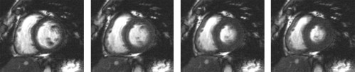
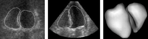
Segmentation of Cardiac MRI Cine Sequences
Get Radiology Tree app to read full this article<
Get Radiology Tree app to read full this article<
Get Radiology Tree app to read full this article<
Get Radiology Tree app to read full this article<
Get Radiology Tree app to read full this article<
CD(SegA,SegB)=2|SegA∩SegB||SegA|+|SegB|. C
D
(
S
e
g
A
,
S
e
g
B
)
=
2
|
S
e
g
A
∩
S
e
g
B
|
|
S
e
g
A
|
+
|
S
e
g
B
|
.
Get Radiology Tree app to read full this article<
Get Radiology Tree app to read full this article<
H(A,B)=max{h→(A,B),h→(B,A)} H
(
A
,
B
)
=
max
{
h
→
(
A
,
B
)
,
h
→
(
B
,
A
)
}
with
h→(A,B)=maxa∈Aminb∈Bd(a,b) h
→
(
A
,
B
)
=
max
a
∈
A
min
b
∈
B
d
(
a
,
b
)
where A and B denote two sets of points of the surface of the two segmentations. D(a, b) is the Euclidean distance between two points ( ). The Hausdorff distance can be interpreted as the maximum difference between the two segmentations.
Get Radiology Tree app to read full this article<
Get Radiology Tree app to read full this article<
Get Radiology Tree app to read full this article<
Table 1
Computed Volumes for the Different Segmentation Models for all 10 Cardiac Magnetic Resonance Imaging Cine Dataset in mL
DS#M 1__M 2__SA 1 EDV ESV EDV ESV EDV ESV 1 142.52 74.60 145.95 50.45 107.16 41.13 2 227.49 143.26 200.35 122.49 173.48 114.80 3 184.24 117.52 150.89 99.65 121.91 72.51 4 143.06 54.93 114.55 21.10 89.51 13.66 5 148.80 70.20 132.24 43.12 108.34 41.77 6 175.89 120.53 116.23 73.83 120.49 83.05 7 381.63 244.05 346.76 221.83 292.82 189.96 8 143.49 80.92 129.82 45.16 99.00 39.88 9 144.41 61.62 121.80 45.94 100.54 50.62 10 236.98 180.03 203.36 144.63 203.80 161.95
Note.—DS = dataset; EDV = end-diastolic volume; ESV = end-systolic volume.
Get Radiology Tree app to read full this article<
Get Radiology Tree app to read full this article<
Table 2
Mean Absolute Difference and Standard Deviation σ for the Volumes Computed from the Different Segmentations of the Cardiac Magnetic Resonance Imaging Cine Sequences in mL
M 2 − M 1__SA 1 − M 1__SA 1 − M 2|ΔEDV|¯¯¯¯¯¯¯¯¯¯¯¯ |
Δ
E
D
V
|
¯ 27.34 51.15 25.43σEDV 15.19 16.19 15.38|ΔESV|¯¯¯¯¯¯¯¯¯¯¯¯ |
Δ
E
S
V
|
¯ 27.95 33.83 12.13σESV 9.74 12.84 10.10
Note.—EDV = end-diastolic volume; ESV = end-systolic volume.
Get Radiology Tree app to read full this article<
Get Radiology Tree app to read full this article<
Get Radiology Tree app to read full this article<
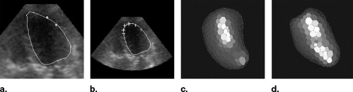
Segmentation of Live 3D Echocardiographic Images
Get Radiology Tree app to read full this article<
Get Radiology Tree app to read full this article<
Get Radiology Tree app to read full this article<
Get Radiology Tree app to read full this article<
Get Radiology Tree app to read full this article<
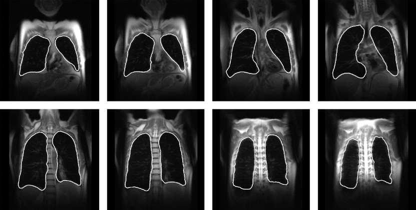
MRI Lung Segmentation
Get Radiology Tree app to read full this article<
Get Radiology Tree app to read full this article<
Get Radiology Tree app to read full this article<
Get Radiology Tree app to read full this article<
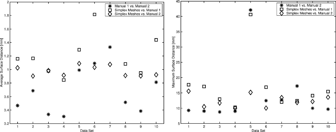
Get Radiology Tree app to read full this article<
Get Radiology Tree app to read full this article<
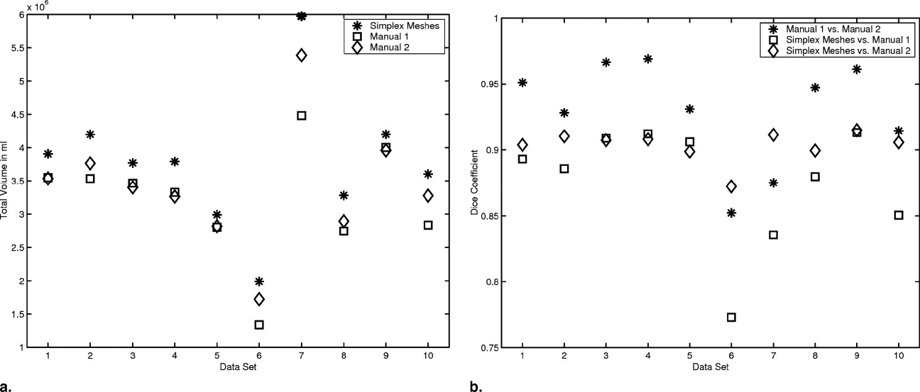
Get Radiology Tree app to read full this article<
Get Radiology Tree app to read full this article<
Get Radiology Tree app to read full this article<
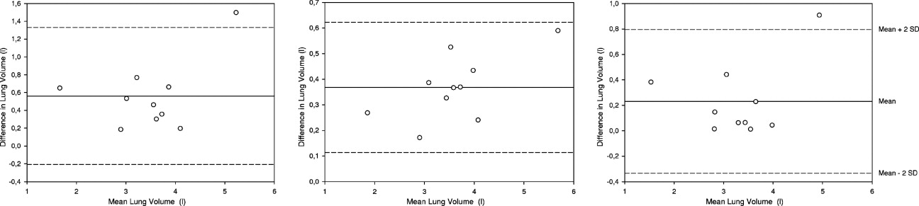
Get Radiology Tree app to read full this article<
Discussion
Get Radiology Tree app to read full this article<
Segmentation of Cardiac Images
Get Radiology Tree app to read full this article<
Get Radiology Tree app to read full this article<
Get Radiology Tree app to read full this article<
Get Radiology Tree app to read full this article<
Segmentation of Pulmonary MRI Data
Get Radiology Tree app to read full this article<
Get Radiology Tree app to read full this article<
Outlook
Get Radiology Tree app to read full this article<
Get Radiology Tree app to read full this article<
Get Radiology Tree app to read full this article<
Acknowledgments
Get Radiology Tree app to read full this article<
Get Radiology Tree app to read full this article<
References
1. Kass M., Witkin A., Terzopoulos D.: Snakes: active contour models. Int J Computer Vision 1988; 1: pp. 321-331.
2. McInerney T., Terzopoulos D.: Topology adaptive deformable surfaces for medical image volume segmentation. Imaging 1999; 18: pp. 840-850.
3. Neuenschwander W., Fua P., Szekely G., et. al.: Deformable Velcro surfaces.Lemke H.Vannier M.Inamura K. et. al.Proceedings of the International Conference on Computer Vision Cambridge.1995.pp. 828-833.
4. Delingette H.: General object reconstruction based on simplex meshes. Int J Computer Vision 1999; 32: pp. 111-146.
5. McInerney T., Terzopoulos D.: Deformable models in medical image analysis: a survey. Med Image Analysis 1996; 1: pp. 1-18.
6. Montagnat J., Delingette H.: A review of deformable surfaces: topology, geometry and deformation. Image Vision Computing 2001; 19: pp. 1023-1040.
7. Cootes T., Taylor C.: Active shape models—smart snakes.Proceedings of the British Machine Vision Conference.1992.Springer VerlagHeidelberg:pp. 266-275.
8. Cootes T.F., Hill A., Taylor C.J., et. al.: The use of active shape models for locating structures in medical images. IPMI 1993; pp. 33-47.
9. Bardinet E., Cohen L., Ayache N.: Superquadrics and free-form deformations: a global model to fit and track 3D medical data.Proceedings of the Conference on Computer Vision, Virtual Reality and Robotics in Medicine (CVRMed ’95) Lecture Notes in Computer Science.1995.Springer VerlagNice, France:pp. 319-326.
10. Terzopoulos D., Metaxas D.: Dynamic 3D deformable models with local and global deformations: deformable superquadrics. IEEE Trans Pattern Analysis Machine Intell 1991; 13: pp. 703-714.
11. Olabarriaga S.D., Smeulders A.W.M.: Interaction in the segmentation of medical images: a survey. Med Image Analysis 2001; 5: pp. 127-142.
12. Cates J., Lefohn A., Whitaker R.: Gist: an interactive, GPU-based level set segmentation tool for 3d medical images. Med Image Analysis 2004; 8: pp. 217-231.
13. Montagnat J., Sermesant M., Delingette H., et. al.: Anisotropic filtering for model based segmentation of 4d cylindrical echocardiographic images. Pattern Recog Lett 2003; 24: pp. 815-828.
14. Montagnat A., Delingette H.: Spatial and temporal shape constrained deformable surfaces for 3D and 4D medical image segmentation.2000.
15. Cohen L.D., Cohen I.: Finite-element method for active contour models and balloons for 2D and 3D images. IEEE Trans Pattern Analysis Machine Intell 1993; 15: pp. 1131-1147.
16. Ibanez L, Schroeder W, Ng L, et al. The ITK software guide. Insight Software Consortium, 2003. Available online at: http://www.itk.org/ItkSoftwareGuide.pdf
17. Böttger T., Kunert T., Meinzer H., et. al.: Interactive constraints for 3D simplex meshes. Medical Imaging 2005: Image Processing SPIE 2005; 5747: pp. 1692-1702.
18. Kunert T., Cardenas C.E., Diehl S., et. al.: Problems of interactive segmentation. Biomedizinische Technik 2002; 47: pp. 933-935.
19. Wolf I., Vetter M., Wegner I., et. al.: The Medical Imaging Interaction Toolkit (MITK)—a toolkit facilitating the creation of interactive software by extending VTK and ITK. Med Imaging Image Proc SPIE 2004; 5367: pp. 16-27.
20. Lethimonnier F., Furber A., Balzer P., et. al.: Global left ventricular cardiac function: comparison between magnetic resonance imaging, radionuclide angiography, and contrast angiography. Invest Radiol 1999; 34: pp. 199-203.
21. Dice L.: Measures of the amount of ecologic association between species. J Ecol 1945; 26: pp. 297-302.
22. Huttenlocher D.P., Klanderman G.A., Rucklidge W.A.: Comparing images using the hausdorff distance. IEEE Trans Pattern Anal Mach Intell 1993; 15: pp. 850-863.
23. Veltkamp R.C.: Shape matching: similarity measures and algorithms.SMI ’01: Proceedings of the International Conference on Shape Modeling & Applications.2001.IEEE Computer SocietyWashington, DC:pp. 188-199.
24. Chan T., Vese L.: Active contours without edges. IEEE Trans Med Image Proc 2001; 10: pp. 266-277.
25. Meyer F., Coifman R.: Brushlets: a tool for directional image analysis and image compression. Appl Comput Harmonic Analysis 1997; 4: pp. 147-187.
26. Gerard O., Billon A., Rouet J.-M., et. al.: Efficient model-based quantification of left ventricular function in 3-d echocardiography. IEEE Trans Med Imaging 2002; 21: pp. 1059-1068.
27. Ray N., Acton S., Altes T., et. al.: Merging parametric active contours within homogeneous image regions for MRI-based lung segmentation. IEEE Trans Med Imaging 2003; 22: pp. 189-199.