Automated 11 C-PiB Standardized Uptake Value Ratio

Rationale and Objectives

Radiotracers such as 11 C-PiB have enabled the in vivo imaging of amyloid-β plaques in the brain, one of the histopathologic hallmarks of Alzheimer’s disease (AD). Standardized uptake value ratio (SUVR) has become the most common normalization for 11 C-PiB as it does not require dynamic scans or blood sampling. Normalization is performed by computing the ratio of 11 C-PiB retention in the whole brain to that in cerebellar gray matter. However, SUVR is still conducted manually and is time consuming. An automated normalization algorithm is proposed.

Materials and Methods

Sixty participants from the Australian Imaging Biomarkers and Lifestyle (AIBL) study were used to test the developed algorithm and compare it against manual SUVR. The cohort consisted of participants likely to have AD ( n = 20), those with mild cognitive impairment (MCI; n = 20), and normal controls (NC; n = 20). The participants underwent 11 C-PiB PET scans. A subset ( n = 15) also underwent magnetic resonance imaging scans. 11 C-PET scans were segmented using an expectation maximization approach with inhomogeneity correction using three-dimensional cubic B-Splines. A cerebellar region was propagated and constrained by segmentation. Comparisons were made between manual and automated SUVR using regional analysis. Receiver-operating characteristic curves were computed for the task of AD–NC classification. Positron emission tomographic segmentations were also compared to co-registered magnetic resonance images of the same patient.

Results

Significant differences in regional means were observed between manual and automated SUVR. However, these changes were highly correlated ( r > 0.8 for most regions). Significant differences ( P < .05) in regional variances were also observed for the AD and NC subgroups. Area under the curve was 0.84 and 0.89 for manual and automated SUVR, respectively.

Conclusions

The automated normalization technique results in less within-group variance and better discrimination between AD and NC participants.

Radiotracers such as 11 C-PiB ( ), 18 F-FDDNP ( ), 11 C-SB-13 ( ), and 18 F-BAY ( ) have enabled the in vivo imaging of amyloid- β (A β ) plaques in the brain. These studies usually involve the collection not only of molecular imaging data but also of structural data from magnetic resonance imaging (MRI) scans. Such datasets are being collected as part of the Alzheimer’s Disease Neuroimaging Initiative in the United States and the Australian Imaging Biomarkers and Lifestyle. Manual processing is very time consuming, tedious, and subject to inter- and intraobserver variabilities. Moreover, the sheer size of these datasets makes manual processing virtually impossible to conduct. Therefore, automated techniques for these tasks are highly desirable.

Various methods have been proposed for studying 11 C-PiB positron emission tomographic (PET) images. Kinetic compartmental analysis has been used previously ( ) to model the uptake and retention of tracer along with its binding characteristics using partial differential equations. This approach uses arterial plasma radioactivity as an input function, requiring arterial blood sampling to measure unmetabolized tracer in plasma. Arterial blood sampling is uncomfortable for participants and is associated with undesirable side effects, such as bleeding, formation of hematomas, infection, and radiation exposure for persons collecting the samples ( ). Scanning time is also protracted as a dynamic acquisition, typically requiring 60 to 90 minutes to be carried out. Outputs of this approach provide regional kinetic coefficients from which distribution volume (DV) of specific ( V__S ), free tissue ( V__FT ), and nonspecific ( V__NS ) components as well as binding potential; namely, free plasma concentration, total plasma concentration, and nondisplaceable uptake can be calculated. DV is the ratio of concentration of radioligand in tissue to free ligand in plasma, whereas binding potential is directly proportional to the ratio of available binding sites and the apparent equilibrium dissociation constant. Some simpler approaches, such as graphic analysis, can also be applied to the quantification of dynamic data. Graphic analysis offers the advantage of being simple and independent of the actual tissue compartmental configuration.

Get Radiology Tree app to read full this article<

Materials and methods

Get Radiology Tree app to read full this article<

Data and Acquisition

Get Radiology Tree app to read full this article<

Table 1

Demographic Information of the Subjects used in this Study

Alzheimer’s Disease Mild Cognitive Impairment Normal Controls Age 72.9 ± 10.3 73.5 ± 8.6 72.2 ± 6.5 M/F 9/11 7/13 10/10 Mini Mental State Exam 19.6 ± 8.1 26.1 ± 2.4 29.3 ± 1.0 Clinical Dementia Rating 1.2 ± 0.8 0.5 ± 0.2 0.1 ± 0.2 Magnetic resonance imaging 5 5 5

Values expressed as means ± SD. The numbers for magnetic resonance imaging indicate the number of scans for each of the groups that was used in the comparison.

Get Radiology Tree app to read full this article<

SUVR Calculation

Get Radiology Tree app to read full this article<

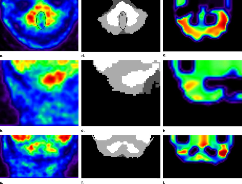
Cerebellar Region Extraction

Get Radiology Tree app to read full this article<

Automatic 11 C-PIB PET Segmentation

Get Radiology Tree app to read full this article<

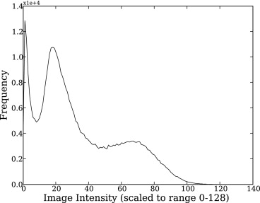
H(Ix)=∑i∈WM,CSF,BCKαiG(σi,μi)+αGMG(σGM,μGM−Bx) H

(

)

∑

∈

(

)

(

−

)

where G ( σ__i__, μ__i ) is a Gaussian function with mean μ__i and standard deviation σ__i describing the intensity distribution of tissue i in the image I__x , and α i the proportion of the i__th tissue.

Get Radiology Tree app to read full this article<

ˆ=argmax(logp(Ix|))

arg

⁡

max

⁡

(

log

⁡

(

)

while estimating the missing data (ie, missing measurements or a hidden variable). The algorithm consists of two steps. The expectation step ( E step) estimates the Q function:

Q(|m)=E[logp(Ix,lx=j|)|Ix,m] Q

(

)

[

log

⁡

(

)

]

where l__x is the tissue label. The M or maximization step maximizes Q :

m+1=argmaxQ(|m) m

arg

⁡

max

⁡

(

)

Maximization of Equation 3 is equivalent to minimizing its negative log. This was the preferred approach as it transforms the multiplicative bias field into an additive one. Within the EM optimization, the 3D cubic B-Spline modeling of heterogeneous GM uptake was iteratively updated, using a set of uniformly spaced controls points in each dimension. On experimentation a knot spacing of 10 mm was found to allow sufficient degrees of freedom to model the complex uptake pattern seen in the GM, without overfitting the brain anatomy. Each of the control points defined a neighborhood of influence ψ t where t indexed the control points. Because we assumed that WM and CSF uptake were homogeneous, the B-Spline modulation was only applied to voxels having a high probability of belonging to GM, that is if:

p(lx=GM|Ix,m)m+1>p(lx=j|Ix,m)m+1∀j∈{WM,CSF,BCK} p

(

)

(

)

∀

∈

{

}

The weighting of the t__th control point, Wmt W

m , at the m__th iteration was computed from its neighborhood as the difference between the global GM mean and the GM mean of the neighborhood, that is Wm+1t=μmGM(Ω)−μmGM(ψt) W

(

)

(

) , where Ω is the domain of the image. The weights of the control points were computed at the end of the M step, and were subsequently used to model the uptake using B-Spline interpolation. The resulting modulation was then applied to all voxels with high probability of being GM.

Get Radiology Tree app to read full this article<

p(lx=j|Ix,m)m+1=p(Ix|lx=j,m)p(lx=j)p(Ix,m)=p(Ix|lx=j,m)p(lx=j)∑Nk=1p(Ix|lx=k,m)p(lx=k)(6) p

(

)

(

)

(

)

(

)

(

)

(

)

∑

(

)

(

)

(

)

where N is the number of tissues.

Get Radiology Tree app to read full this article<

p(Ix|lx=j,m)=G(σj,μj−BxMx) p

(

)

(

−

)

Get Radiology Tree app to read full this article<

μm+1i(Ω)=∑x∈Ωp(lx=i|Ix)(Ix−BxMx)∑x∈Ωp(lx=i|Ix) μ

(

)

∑

∈

(

)

(

−

)

∑

∈

(

)

(σm+1i)2(Ω)=∑x∈Ωp(lx=i|Ix)(Ix−BxMx−μm+1i)2∑x∈Ωp(lx=i|Ix) (

)

(

)

∑

∈

(

)

(

−

)

∑

∈

(

)

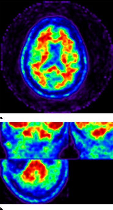
Convergence was achieved when the difference in log likelihood (Eq 2 ) between subsequent iterations is below a threshold (0.0001). A final maximum a posteriori segmentation was then computed from the posterior probabilities ( ) by assigning the class with the highest probability at each voxel. Segmentation results are presented in Figure 3 .

Get Radiology Tree app to read full this article<

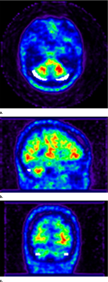
Segmentation Propagation and Cleanup

Get Radiology Tree app to read full this article<

Experimental Methods

Manual SUVR calculation

Get Radiology Tree app to read full this article<

Segmentation validation with MRI

Get Radiology Tree app to read full this article<

DSC=2|SM∩SP||SM|+|SP| DSC

∩

DSC means and standard deviations with each group were calculated and the results are presented in Segmentation Validation with MRI.

Get Radiology Tree app to read full this article<

Comparison to manual SUVR

Get Radiology Tree app to read full this article<

Table 2

Regions Used for Automated Regional Statistics Computation

Combined Region Automated Anatomic Labeling Template Regions Frontal Precentral, frontal superior, frontal superior orbital, frontal mid, frontal mid orbital, frontal inferior oper, frontal inferior tri, frontal superior medial, frontal mid orbital, frontal inferior orbital Lateral temporal Temporal superior, temporal pole superior, temporal mid, temporal pole mid, temporal inferior Medial temporal Amygdala, hippocampus, parahippocampal Occipital Occipital superior, occipital mid, occipital inferior Parietal Parietal superior, parietal inferior Precuneus Precuneus Posterior cingulate Cingulum posterior Anterior cingulated Cingulum anterior Caudate Caudate

Combined regions are presented in column 1 and their corresponding automated anatomic labelling template regions are presented in column 2.

Get Radiology Tree app to read full this article<

d=μAD−μNCσpooledwhereσpooled=σ2AD+σ2NC2−−−−−−−√ d

−

where

where μ__AD and σ__AD refer to the ROI means and standard deviation, respectively, for AD participants (similarly for normal controls: μ__NC and σ__NC ). The metric measures the size of observed effects, whether they are statistically significant or not. In this case, the metric can be interpreted as a measure of the ability of a binary classifier to distinguish between AD and NC subjects based on uptake with higher effect sizes leading to better separation. The metric was computed for all regions.

Get Radiology Tree app to read full this article<

Results

Segmentation Validation with MRI

Get Radiology Tree app to read full this article<

Table 3

Dice Scores of Comparison Between Magnetic Resonance Imaging and Positron Emission Tomographic Segmentations

Gray Matter White Matter Alzheimer’s disease 0.75 ± 0.02 0.85 ± 0.02 Mild cognitive impairment 0.73 ± 0.02 0.78 ± 0.08 Normal controls 0.72 ± 0.02 0.77 ± 0.04

Values presented as mean ± SD.

Get Radiology Tree app to read full this article<

Regional Analysis of Automated and Manual SUVR

Get Radiology Tree app to read full this article<

Table 4

Standardized Uptake Value Ratio Results for Automated vs. Manual Analysis

Classification Manual AD MCI NC Automatic AD MCI NC Anterior cingulate 2.17 (21.7) 1.83 (30.1) 1.51 (14.7) 1.88 (13.3) ⁎ 1.62 (25.2) 1.39 (10.3) ⁎ Caudate 1.51 (28.0) 1.26 (33.1) 1.22 (19.1) 1.30 (19.8) 1.11 (26.1) 1.12 (16.4) Frontal 1.96 (18.8) 1.63 (31.3) 1.23 (14.3) 1.70 (10.1) ‡ 1.44 (26.0) 1.13 (9.9) ⁎ Lateral temporal 1.86 (19.0) 1.64 (30.2) 1.23 (14.1) 1.61 (8.5) † 1.45 (25.1) 1.13 (9.4) ⁎ Medial temporal 1.41 (17.5) 1.38 (16.4) 1.30 (9.2) 1.23 (9.5) ‡ 1.23 (9.2) ⁎ 1.19 (4.8) ‡ Occipital 1.80 (23.4) 1.60 (21.6) 1.36 (14.1) 1.55 (12.0) ⁎ 1.42 (18.1) 1.24 (8.9) ⁎ Parietal 1.85 (21.0) 1.46 (32.1) 1.10 (17.6) 1.60 (12.7) † 1.29 (27.6) 1.00 (12.2) ⁎ Posterior cingulate 1.91 (23.9) 1.73 (23.6) 1.64 (15.5) 1.65 (16.3) 1.53 (17.0) 1.50 (10.7) ⁎ Precuneus 2.14 (19.3) 1.73 (30.7) 1.27 (18.6) 1.85 (8.3) ‡ 1.53 (26.4) 1.16 (13.4) ⁎

AD, Alzheimer’s disease; MCI, mild cognitive impairment; NC, normal controls.

Values presented as mean (coefficient of variation). The f -test was conducted between the same group of the different methods.

f -test:

Get Radiology Tree app to read full this article<

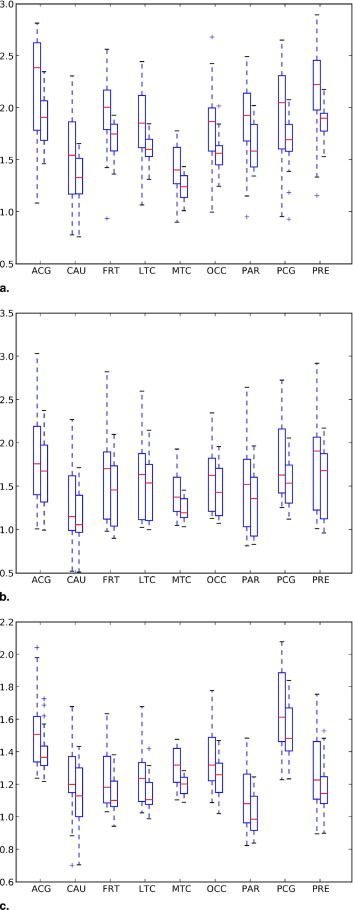
Table 5

Correlation Coefficients Between Manual and Automated Analysis

Alzheimer’s Disease Mild Cognitive Impairment Normal Controls_r__r__r_ Anterior cingulate 0.78 0.94 0.90 Caudate 0.87 0.95 0.93 Frontal 0.68 0.93 0.90 Lateral temporal 0.70 0.93 0.90 Medial temporal 0.54 0.77 0.70 Occipital 0.86 0.85 0.90 Parietal 0.78 0.93 0.94 Posterior cingulate 0.78 0.90 0.92 Precuneus 0.77 0.93 0.94

The coefficients of determination are the square of r .

Get Radiology Tree app to read full this article<

Table 6

Effect Size of the Two Methods for a Set of Selected Regions

Manual Auto Anterior cingulate 1.78 2.38 Caudate 0.83 0.79 Frontal 2.51 3.90 Lateral temporal 2.24 3.90 Medial temporal 0.58 0.37 Occipital 1.37 2.03 Parietal 2.45 3.54 Posterior cingulate 0.74 0.68 Precuneus 2.60 4.45

The effect size was measured between Alzheimer’s disease and normal controls for each of the two methods.

Get Radiology Tree app to read full this article<

Discussion

Get Radiology Tree app to read full this article<

Conclusions

Get Radiology Tree app to read full this article<

References

1. Klunk W.E., Engler H., Nordberg A., et. al.: Imaging brain amyloid in Alzheimer’s disease with Pittsburgh Compound-B. Ann Neurol 2004; 55: pp. 306-319.
2. Agdeppa E.D., Kepe V., Liu J., et. al.: Binding characteristics of radiofluorinated 6-dialkylamino-2-naphthylethylidene derivatives as positron emission tomography imaging probes for beta-amyloid plaques in Alzheimer’s disease. J Neurosci 2001; 21: pp. 1-5.
3. Verhoeff N.P., Wilson A.A., Takeshita S., et. al.: In-vivo imaging of Alzheimer disease beta-amyloid with [11C]SB-13 PET. Am J Geriat Psychiatry 2004; 12: pp. 584-595.
4. Rowe C.C., Ackerman U., Browne W., et. al.: Imaging of amyloid β in Alzheimer’s disease with 18F-BAY94-9172, a novel PET tracer: proof of mechanism. Lancet Neurol 2008; 7: pp. 129-135.
5. Price J.C., Klunk W.E., Lopresti J., et. al.: Kinetic modeling of amyloid binding in humans using PET imaging and Pittsburgh Compound-B. B. J Cereb Blood Flow Metab 2005; 25: pp. 1528-1547.
6. Jons P.H., Ernst M., Hankerson J., et. al.: Follow-up of radial arterial catheterization for positron emission tomography studies. Hum Brain Mapp 1997; 5: pp. 119-123.
7. Logan J., Fowler J.S., Volkow N.D., et. al.: Graphical analysis of reversible radioligand binding from time-activity measurements applied to [N-11C-methyl]-(-)-cocaine PET studies in human subjects. J Cereb Blood Flow Metab 1990; 10: pp. 740-747.
8. Logan J., Fowler J.S., Volkow N.D., et. al.: Distribution volume ratios without blood sampling from graphical analysis of PET data. J Cereb Blood Flow Metab 1996; 16: pp. 834-840.
9. Lopresti B.J., Klunk W.E., Mathis C.A., et. al.: Simplified quantification of Pittsburgh compound B amyloid imaging PET studies: a comparative analysis. J Nucl Med 2005; 46: pp. 1959-1972.
10. Joachim C., Morris J., Selkoe D.: Diffuse senile plaques occur commonly in the cerebellum in Alzheimer’s disease. Am J Pathol 1989; 135: pp. 309-319.
11. Rowe C.C., Ng S., Ackermann U., et. al.: Imaging beta-amyloid burden in aging and dementia. Neurology 2007; 68: pp. 1718-1725.
12. Lockhart A., Lamb J., Osredkar T., et. al.: PIB is a non-specific imaging marker of amyloid-beta (Abeta) peptide-related cerebral amyloidosis. Brain 2007; 130: pp. 2607-2615.
13. Edison P., Archer H.A., Hinz R., et. al.: Amyloid, hypometabolism, and cognition in Alzheimer disease: an [11C]PIB and [18F]FDG PET study. Neurology 2007; 68: pp. 501-508.
14. Fagan A.M., Mintun M.A., Mach R.H., et. al.: Inverse relation between in vivo amyloid imaging load and cerebrospinal fluid Abeta42 in humans. Ann Neurol 2006; 59: pp. 512-519.
15. Kemppainen N.M., Aalto S., Wilson I.A., et. al.: PET amyloid ligand [11C]PIB uptake is increased in mild cognitive impairment. Neurology 2007; 68: pp. 1603-1606.
16. Yasuno F., Hasnine A.H., Suhara T., et. al.: Template-based method for multiple volumes of interest of human brain PET images. NeuroImage 2002; 16: pp. 577-586.
17. Mykkänen J., Tohka J., Luoma J., et. al.: Automatic extraction of brain surface and mid-sagittal plane from PET images applying deformable models. Comput Methods Programs Biomed 2005; 79: pp. 1-17.
18. Tohka J.: Surface extraction from volumetric images using deformable meshes: a comparative study.2002.pp. 350-364. In: European Conference on Computer Vision–ECCV 2002. Copenhagen, Denmark May 28–31, 2002.
19. Chen J.L., Gunn S.R., Nixon M.S., et. al.: Markov random field models for segmentation of PET images.2001.pp. 468-474. In: Information processing in Medical Imaging, 17th International Conference, IPMI. Davis, CA, June 18–22, 2001.
20. Wong D.P., Feng D., Meikle S.R., et. al.: Segmentation of dynamic PET images using cluster analysis. IEEE Trans Nucl Sci 2002; 49: pp. 200-207.
21. Brankov J.G., Galatsanos N.P., Yang Y., et. al.: Segmentation of dynamic PET or fMRI images based on a similarity metric. IEEE Trans Nucl Sci 2003; 50: pp. 1410-1414.
22. Koivistoinen H., Tohka J., Ruotsalainen U.: Comparison of pattern classification methods in segmentation of dynamic PET brain images. 6th Nordic Signal Processing Symposium, IEEE 2004; pp. 73-76.
23. Browne J., de Pierro A.: A row-action alternative to the EM algorithm for maximizing likelihood in emission tomography. IEEE Trans Med Imaging 1996; 15: pp. 687-699.
24. Folstein M.F., Folstein S.E., McHugh P.R.: Mini-mental state. J Psychiatr Res 1975; 12: pp. 189-198.
25. Morris J.C.: The Clinical Dementia Rating (CDR): current version and scoring rules. Neurology 1993; 43: pp. 2412-2414.
26. Raniga P., Bourgeat P., Villemagne V., et. al.: Spline based inhomogeneity correction for [11]C-PIB PET segmentation using expectation maximization.Ayache N.Ourselin S.Maeder A.2007.SpringerBerlin, Germany:pp. 228-235.
27. Aston J.A.D., Cunningham V.J., Asselin M.C., et. al.: Positron emission tomography partial volume correction: estimation and algorithms. J Cereb Blood Flow Metab 2002; 22: pp. 1019-1034.
28. Lamare F., Turzo A., Bizais Y., et. al.: Validation of a Monte Carlo simulation of the Philips Allegro/GEMINI PET systems using GATE. Phys Med Biol 2006; 51: pp. 943-962.
29. Dempster A.P., Laird N.M., Rubin D.B.: Maximum likelihood from incomplete data via the EM algorithm. J Roy Stat Soc 1977; 39: pp. 1-38.
30. Mazziotta J., Toga A., Evans A., et. al.: A probabilistic atlas and reference system for the human brain: International Consortium for Brain Mapping (ICBM). Philos Trans R Soc Lond B Biol Sci 2001; 356: pp. 1293-1322.
31. Ourselin S., Roche A., Subsol G., et. al.: Reconstructing a 3D structure from serial histological sections. Image Vision Computing 2001; 19: pp. 25-31.
32. Kang Y., Engelke K., Kalender W.A.: Interactive 3D editing tools for image segmentation. Med Image Anal 2004; 8: pp. 35-46.
33. Ibanez L., Schroeder W., Ng L., et. al.: The ITK Software Guide, Kitware, Inc.. http://www.itk.org/ItkSoftwareGuide.pdf 2nd ed, 2005. Accessed December 15, 2007.
34. Van Leemput K., Maes F., Vandermeulen D., et. al.: Automated model-based tissue classification of MR images of the brain. IEEE Trans Med Imaging 1999; 18: pp. 897-908.
35. Dice L.: Measures of the amount of ecologic association between species. Ecology 1945; 26: pp. 297-302.
36. Kim J., Cai W., Feng D., et. al.: Segmentation of VOI from multidimensional dynamic PET images by integrating spatial and temporal features. IEEE Trans Info Technol Biomed 2006; 10: pp. 637-646.
37. Tzourio-Mazoyer N., Landeau B., Papathanassiou D., et. al.: Automated anatomical labeling of activations in SPM using a macroscopic anatomical parcellation of the MNI MRI single-subject brain. NeuroImage 2002; 15: pp. 273-289.
38. Development Core Team, R:a language and environment for statistical computing. http://www.R-project.org Accessed January 4, 2008.
39. Metz C.E., Herman B.A., Roe C.A.: Statistical comparison of two ROC-curve estimates obtained from partially-paired datasets. Med Decis Making 1998; 18: pp. 110-121.
40. Cohen J.: Statistical power analysis for the behavioral sciences.2nd ed.1988.Lawrence Erlbaum AssociatesHillsdale, NJ
41. Rosnow R.L., Rosenthal R.: Computing contrasts, effect sizes, and counternulls on other people’s published data: general procedures for research consumers. Psychol Meth 1996; 1: pp. 331-340.

Automated 11 C-PiB Standardized Uptake Value Ratio

Rationale and Objectives

Materials and Methods

Results

Conclusions

Materials and methods

Data and Acquisition

SUVR Calculation

Cerebellar Region Extraction

Automatic 11 C-PIB PET Segmentation

Segmentation Propagation and Cleanup

Experimental Methods

Manual SUVR calculation

Segmentation validation with MRI

Comparison to manual SUVR

Results

Segmentation Validation with MRI

Regional Analysis of Automated and Manual SUVR

Discussion

Conclusions

References

Further Reading

Abstracts of Funded National Institutes of Health Grants

Advances in Radiological Image Analysis from MICCAI 2007

Automated Segmentation of the Liver from 3D CT Images Using Probabilistic Atlas and Multilevel Statistical Shape Model