Automated Breast Segmentation of Fat and Water MR Images Using Dynamic Programming

Rationale and Objectives

To develop and test an algorithm that outlines the breast boundaries using information from fat and water magnetic resonance images.

Materials and Methods

Three algorithms were implemented and tested using registered fat and water magnetic resonance images. Two of the segmentation algorithms are simple extensions of the techniques used for contrast-enhanced images: one algorithm uses clustering and local gradient (CLG) analysis and the other algorithm uses a Hessian-based sheetness filter (HSF). The third segmentation algorithm uses k-means++ and dynamic programming (KDP) for finding the breast pixels. All three algorithms separate the left and right breasts using either a fixed region or a morphological method. The performance is quantified using a mutual overlap (Dice) metric and a pectoral muscle boundary error. The algorithms are evaluated against three manual tracers using 266 breast images from 14 female subjects.

Results

The KDP algorithm has a mean overlap percentage improvement that is statistically significant relative to the HSF and CLG algorithms. When using a fixed region to remove the tissue between breasts with tracer 1 as a reference, the KDP algorithm has a mean overlap of 0.922 compared to 0.864 ( P < .01) for HSF and 0.843 ( P < .01) for CLG. The performance of KDP is very similar to tracers 2 (0.926 overlap) and 3 (0.929 overlap). The performance analysis in terms of pectoral muscle boundary error showed that the fraction of the muscle boundary within three pixels of reference tracer 1 is 0.87 using KDP compared to 0.578 for HSF and 0.617 for CLG. Our results show that the performance of the KDP algorithm is independent of breast density.

Conclusions

We developed a new automated segmentation algorithm (KDP) to isolate breast tissue from magnetic resonance fat and water images. KDP outperforms the other techniques that focus on local analysis (CLG and HSF) and yields a performance similar to human tracers.

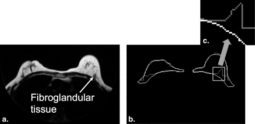
Breast density (BD) is a known risk factor for the development of breast cancer . BD is routinely measured in mammography by comparing the ratio of stromal tissue to fatty tissue. Radiologists typically visually estimate BD from mammograms according to four categories: almost entirely fatty, scattered areas of fibroglandular densities, heterogeneously dense, or extremely dense . Because increased BD (including the heterogeneously dense or extreme dense categories) is associated with a higher risk for breast cancer, therapies that reduce BD have been proposed as cancer preemptive treatments . For studies assessing the effect of BD reduction therapies, it is desirable to follow changes in BD longitudinally. Unfortunately, the radiation exposure in mammography makes the technique impractical for serial studies of BD. Mammograms also yield two-dimensional information and the densities may change based on the projection, level and angle of compression, and scanner calibration .

Magnetic resonance imaging (MRI) is a noninvasive three-dimensional (3D) imaging technique that uses nonionizing radiation. More importantly, MRI yields distinct fat and water signals; thus, the technique is an alternative to the mammographic measurement of BD. In recent years, several MRI techniques have been developed for the measurement of fat–water content. These techniques are based on the acquisition of data where fat and water spins have different relative phases; the data are processed to reconstruct fat and water images corrected for the effect of field inhomogeneities . In this study, we use one of these techniques: the radial gradient-echo and spin-echo (RADGRASE) technique. RADGRASE yields fat, water, and T2-corrected fat-fraction (FF) images for the entire breast (approximately nineteen 7-mm thick slices) from data acquired in only 3 minutes . Parameters derived from the FF distribution in the breast have showed a high correlation with mammography BD . To analyze BD in the breast, the first step is to define a region of interest (ROI) by segmenting the breast from the rest of the image. The manual segmentation of a stack of breast image slices is time consuming and impractical.

Get Radiology Tree app to read full this article<

Materials and methods

Data Acquisition

Get Radiology Tree app to read full this article<

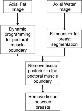
Automatic Segmentation Algorithm

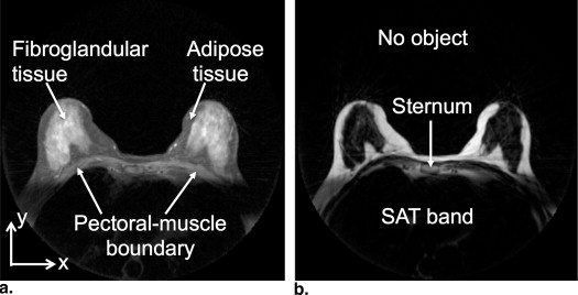
Features in the Fat and Water Images

Get Radiology Tree app to read full this article<

Step 1: Initial Breast Segmentation

Get Radiology Tree app to read full this article<

Step 2: Pectoral Muscle Boundary Delineation

Get Radiology Tree app to read full this article<

C(x,y)=−ⅆIF(x,y)dy, C

(

)

−

ⅆ

(

)

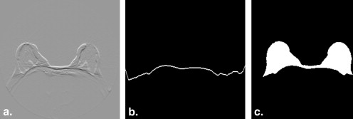
which is applied to the fat image ( Fig 5 a). This cost function outlines the bright-to-dark transitions in the fat image. A similar cost function was used by Giannini et al. to find the pectoral muscle boundary. Using this cost function, the dynamic programming algorithm finds the minimum-cost path through the fat image, that is, the path that maximizes the sum of the vertical derivatives values, dIF(x,y)dy d

(

)

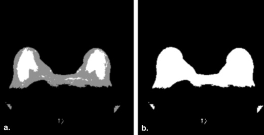
y , estimated in the discrete image using the well-known first-difference calculation, I__F ( x , y ) − I__F ( x , y − 1). Dynamic programming requires a starting point that is set to the highest vertical derivative value in the sternum region, as described previously. The path begins at the starting point and goes left and right, outlining the pectoral muscle boundary ( Fig 5 b). Since we know that the pixels posterior to the pectoral boundary are not part of the breast, we refine the initial breast segmentation mask ( Fig 4 b) by setting those pixels to zero ( Fig 5 c).

Get Radiology Tree app to read full this article<

Step 3: Removing the Chest Tissue

Get Radiology Tree app to read full this article<

Manual Tracing Protocol

Get Radiology Tree app to read full this article<

Extension of Other Algorithms to Fat–Water Images

Get Radiology Tree app to read full this article<

Performance Metrics

Get Radiology Tree app to read full this article<

Dice Metric

Get Radiology Tree app to read full this article<

2|X∩Y||X|+|Y| 2

∩

Get Radiology Tree app to read full this article<

Pectoral Muscle Boundary Difference

Get Radiology Tree app to read full this article<

Analysis Tools

Hypothesis Testing

Get Radiology Tree app to read full this article<

t=μ1−μ2s21N1+s22N2√, t

−

where μ 1 and s 1 are the mean and standard deviation of a first algorithm and μ 2 and s 2 are the mean and standard deviation of a second algorithm. For our experiments, the number of image slices analyzed is N 1 = N 2 = 266. A t statistic of 2.34 would yield a P value of .01, which indicates that μ 1 > μ 2 with 99% confidence interval (ie, a one-tailed test).

Get Radiology Tree app to read full this article<

Cumulative Distribution Function Analysis

Get Radiology Tree app to read full this article<

Results

Get Radiology Tree app to read full this article<

Table 1

Inter-Tracer Performance (Dice Metric)

Tracer #1 Tracer #2 Tracer #3 μ ∗ σ † μ σ μ σ Tracer #1 — — 0.926 0.046 0.929 0.054 Tracer #2 0.926 0.046 — — 0.902 0.070 Tracer #3 0.929 0.054 0.902 0.070 — —

Get Radiology Tree app to read full this article<

Table 2

Automatic Segmentation Performance (Dice Metric)

Method Splitting Technique Tracer #1 Tracer #2 Tracer #3 μ ∗ σ † μ σ μ σ KDP FSRM 0.922 0.047 0.910 0.052 0.908 0.067 MSRM 0.897 0.114 0.878 0.123 0.899 0.107 HSF FSRM 0.864 0.079 0.846 0.082 0.860 0.083 MSRM 0.847 0.095 0.827 0.100 0.852 0.092 CLG FSRM 0.843 0.107 0.830 0.109 0.835 0.119 MSRM 0.833 0.113 0.817 0.121 0.831 0.119

CLG, clustering and local gradient; FSRM, fixed sternum removal method; KDP, k-means++ and dynamic programming; HSF, Hessian-based sheetness filter; MSRM, morphological sternum removal method.

Get Radiology Tree app to read full this article<

Table 3

T Score/ P Value Using Dice Metric

Methods Splitting Technique Tracer #1 Tracer #2 Tracer #3t Score_P_ Value_t_ Score_P_ Value_t_ Score_P_ Value KDP versus HSF FSRM 10.25 <.01 10.60 <.01 7.25 <.01 MSRM 5.49 <.01 5.14 <.01 5.44 <.01 KDP versus CLG FSRM 11.00 <.01 10.78 <.01 8.69 <.01 MSRM 6.52 <.01 5.70 <.01 6.88 <.01

CLG, clustering and local gradient; FSRM, fixed sternum removal method; KDP, k-means++ and dynamic programming; HSF, Hessian-based sheetness filter; MSRM, morphological sternum removal method.

Get Radiology Tree app to read full this article<

Table 4

Pectoral Muscle Boundary CDF

Difference ∗ (pixels) 0 ≤1 ≤2 ≤3 ≤4 ≤5 ≤10 ≤20 ≤50 Tracer #2 — 0.202 0.552 0.757 0.848 0.895 0.925 0.983 0.999 1.000 Tracer #3 — 0.253 0.624 0.797 0.866 0.901 0.926 0.981 0.998 1.000 KDP FSRM 0.071 0.375 0.748 0.870 0.912 0.938 0.988 0.999 1.000 MSRM 0.054 0.334 0.713 0.841 0.892 0.922 0.982 0.997 1.000 HSF FSRM 0.025 0.159 0.438 0.578 0.631 0.671 0.828 0.967 1.000 MSRM 0.019 0.140 0.419 0.567 0.625 0.666 0.820 0.959 0.999 CLG FSRM 0.059 0.285 0.528 0.617 0.660 0.692 0.803 0.932 0.999 MSRM 0.066 0.302 0.546 0.631 0.673 0.704 0.813 0.937 0.999

CDF, cumulative distribution function; CLG, clustering and local gradient; FSRM, fixed sternum removal method; KDP, k-means++ and dynamic programming; HSF, Hessian-based sheetness filter; MSRM, morphological sternum removal method.

Get Radiology Tree app to read full this article<

Discussion

Get Radiology Tree app to read full this article<

Conclusions

Get Radiology Tree app to read full this article<

Acknowledgment

Get Radiology Tree app to read full this article<

References

1. Wolfe J.N.: Risk for breast cancer development determined by mammographic parenchymal pattern. Cancer 1976; 5: pp. 2486-2492.
2. Sandberg M.E., Li J., Hall P., et. al.: Change of mammographic density predicts the risk of contralateral breast cancer—a case-control study. Breast Cancer Res 2013; 15: pp. R57.
3. Pinto Pereira S.M., McCormack V.A., Hipwell J.H., et. al.: Localized fibroglandular tissue as a predictor of future tumor location within the breast. Cancer Epidemiol Biomarkers Prev 2011; 20: pp. 1718-1725.
4. McCormack V.A., dos Santos Silva I.: Breast density and parenchymal patterns as markers of breast cancer risk: a meta-analysis. Cancer Epidemiol Biomarkers Prev 2006; 15: pp. 1159-1169.
5. Burnside E.S., Sickles E.A., Bassett L.W., et. al.: The ACR BI-RADS experience: learning from history. J Amer Col Radiol 2009; 12: pp. 851-860.
6. Li J., Humphreys K., Eriksson L., et. al.: Mammographic density reduction is a prognostic marker of response to adjuvant tamoxifen therapy in postmenopausal patients with breast cancer. J Clin Oncol 2013; 31: pp. 2249-2256.
7. Cuzick J., Warwick J., Pinney E., et. al.: Tamoxifen-induced reduction in mammographic density and breast cancer risk reduction: a nested case-control study. J Natl Cancer Inst 2011; 103: pp. 744-752.
8. McTiernan A., Martin C.F., Peck J.D., et. al.: Estrogen-plus-progestin use and mammographic density in postmenopausal women: women’s health initiative randomized trail. J Natl Cancer Inst 2005; 97: pp. 1366-1376.
9. Ortiz C.G.: Automatic 3D segmentation of the breast in MRI. M.S. thesis2011.Department of Medical Biophysics, University of TorontoToronto, Canada
10. Li Z., Graff C., Gmitro A.F., et. al.: Rapid water and lipid imaging with T2 mapping using a radial IDEAL-GRASE technique. Magnet Reson Med 2009; 6: pp. 1415-1424.
11. Clendenen T.V., Zeleniuch-Jacquotte A., May L., et. al.: Comparison of 3-point Dixon imaging and fuzzy C-means clustering methods for breast density measurement. J Magn Reson Im 2013; 38: pp. 474-481.
12. Wang Y., Morrell G., Heibrun M.E., et. al.: 3D multi-parametric breast MRI segmentation using hierarchical support vector machine with coil sensitivity correction. Acad Radiol 2013; 20: pp. 137-147.
13. Ma J.F., Son J.B., Zhou Y., et. al.: Fast spin-echo triple-echo dixon (fTED) technique for efficient T2-weighted water and fat imaging. Magn Reson Med 2007; 58: pp. 103-109.
14. Bley T.A., Wieben O., Francois C.J., et. al.: Fat and water magnetic resonance imaging. J Magn Reson Im 2010; 31: pp. 4-18.
15. Madhuranthakam A.J., Yu H., Shimakawa A., et. al.: T(2)-weighted 3D fast spin echo imaging with water-fat separation in a single acquisition. J Magn Reson Im 2010; 32: pp. 745-751.
16. Trouard T.P., Thompson P., Huang C., et. al.: Fat water ratio and diffusion-weighted MRI applied to the measure of breast density as a cancer risk biomarker. Proc Int Soc Magn Res Med 2010; pp. 4749.
17. Oliver A., Freixenet J., Martí J., et. al.: A review of automatic mass detection and segmentation in mammographic images. Med Image Anal 2010; 2: pp. 87-110.
18. Ganesan K., Acharya U.R., Chua K.C., et. al.: Pectoral muscle segmentation: a review. Comput Meth Prog Bio 2013; 1: pp. 48-57.
19. Nie K., Chen J.H., Chan S., et. al.: Development of a quantitative method for analysis of breast density based on three-dimensional breast MRI. Med Phys 2008; 12: pp. 5253-5262.
20. Ertas G., Gulcur H., Osman O., et. al.: Breast MR segmentation and lesion detection with cellular neural networks and 3D template matching. Comput Biol Med 2008; 1: pp. 116-126.
21. Kass M., Witkin A., Terzopoulos D.: Snakes: active contour models. Int J Comput Vision 1988; 4: pp. 321-331.
22. Xu C., Prince J.L.: Snakes, shapes, and gradient vector flow. IEEE T Image Process 1998; 3: pp. 359-369.
23. Lee N., Rusinek H., Weinreb J., et. al.: Fatty and fibroglandular tissue volumes in breasts of women 20-83 years old: comparison of X-ray mammography and computer-assisted MR imaging. Am J Roentgenol 1997; 2: pp. 501-506.
24. Khazen M., Warren R.M.L., Boggis C.R.M., et. al.: A pilot study of compositional analysis of the breast and estimation of breast mammographic density using three-dimensional T1-weighted magnetic resonance imaging. Cancer Epidem Biomar 2008; 9: pp. 2268-2274.
25. Giannini V., Vignati A., Morra L., et. al.: A fully automatic algorithm for segmentation of the breasts in DCE-MR images. Proc Eng Med Biol Soc 2010; pp. 3146-3149.
26. Wang L., Platel B., Ivanovskaya T., et. al.: Fully automatic breast segmentation in 3D breast MRI. Int Symp Biomed Imaging 2012; pp. 1024-1027.
27. Arthur D., Vassilvitskii S.: K-means++: the advantages of careful seeding. Proceedings of the Eighteenth Annual Association of Computing Machinery-Society for Industrial and Applied Mathematics, Symposium on Discrete Algorithms 2007; pp. 1027-1035.
28. Sonka M., Hlavac V., Boyle R.: Segmentation I.Sonka M.Hlavac V.Boyle R.Image processing, analysis and machine vision.2014.Global EngineeringStanford, CT:pp. 206-210.
29. Rosado-Toro J.A., Barr T., Galons J.P., et. al.: Automated segmentation of breast fat-water MR images using empirical analysis. IEEE Int Conf Acoust Speech Signal Process 2013; pp. 1018-1022.
30. Pal N.R., Bezdek J.C.: On cluster validity for the fuzzy c-means model. IEEE T Fuzzy Syst 1995; 3: pp. 370-379.
31. Timp S., Karssemeijer N.: A new 2D segmentation method based on dynamic programming applied to computer aided detection in mammography. Med Phys 2004; 5: pp. 958-971.
32. Salvador S., Chan P.: Determining the number of clusters/segments in hierarchical clustering/segmentation algorithms. ICTAI 2004; pp. 576-584.
33. Dice L.: Measures of the amount of ecologic association between species. Ecology J 1945; 3: pp. 297-302.
34. Yuen K.K.: The two-sample trimmed t for unequal population variances. Biometrika 1974; 1: pp. 165-170.

Automated Breast Segmentation of Fat and Water MR Images Using Dynamic Programming

Rationale and Objectives

Materials and Methods

Results

Conclusions

Materials and methods

Data Acquisition

Automatic Segmentation Algorithm

Features in the Fat and Water Images

Step 1: Initial Breast Segmentation

Step 2: Pectoral Muscle Boundary Delineation

Step 3: Removing the Chest Tissue

Manual Tracing Protocol

Extension of Other Algorithms to Fat–Water Images

Performance Metrics

Dice Metric

Pectoral Muscle Boundary Difference

Analysis Tools

Hypothesis Testing

Cumulative Distribution Function Analysis

Results

Discussion

Conclusions

Acknowledgment

References

Further Reading

Assessing the Appropriateness of Outpatient Abdominopelvic CT and MRI Examinations Using the American College of Radiology Appropriateness Criteria

Automated Tissue Segmentation in Breast MRI

Computer-Aided Diagnosis for Preoperative Invasion Depth of Gastric Cancer with Dual-Energy Spectral CT Imaging