Automated Method for Identification of Patients With Alzheimer’s Disease Based on Three-dimensional MR Images

Rationale and Objectives

An automated method for identification of patients with cerebral atrophy due to Alzheimer’s disease (AD) was developed based on three-dimensional (3D) T1-weighted magnetic resonance (MR) images.

Materials and Methods

Our proposed method consisted of determination of atrophic image features and identification of AD patients. The atrophic image features included white matter and gray matter volumes, cerebrospinal fluid (CSF) volume, and cerebral cortical thickness determined based on a level set method. The cortical thickness was measured with normal vectors on a voxel-by-voxel basis, which were determined by differentiating a level set function. The CSF spaces within cerebral sulci and lateral ventricles (LVs) were extracted by wrapping the brain tightly in a propagating surface determined with a level set method. Identification of AD cases was performed using a support vector machine (SVM) classifier, which was trained by the atrophic image features of AD and non-AD cases, and then an unknown case was classified into either AD or non-AD group based on an SVM model. We applied our proposed method to MR images of the whole brains obtained from 54 cases, including 29 clinically diagnosed AD cases (age range, 52−82 years; mean age, 70 years) and 25 non-AD cases (age range, 49−78 years; mean age, 62 years).

Results

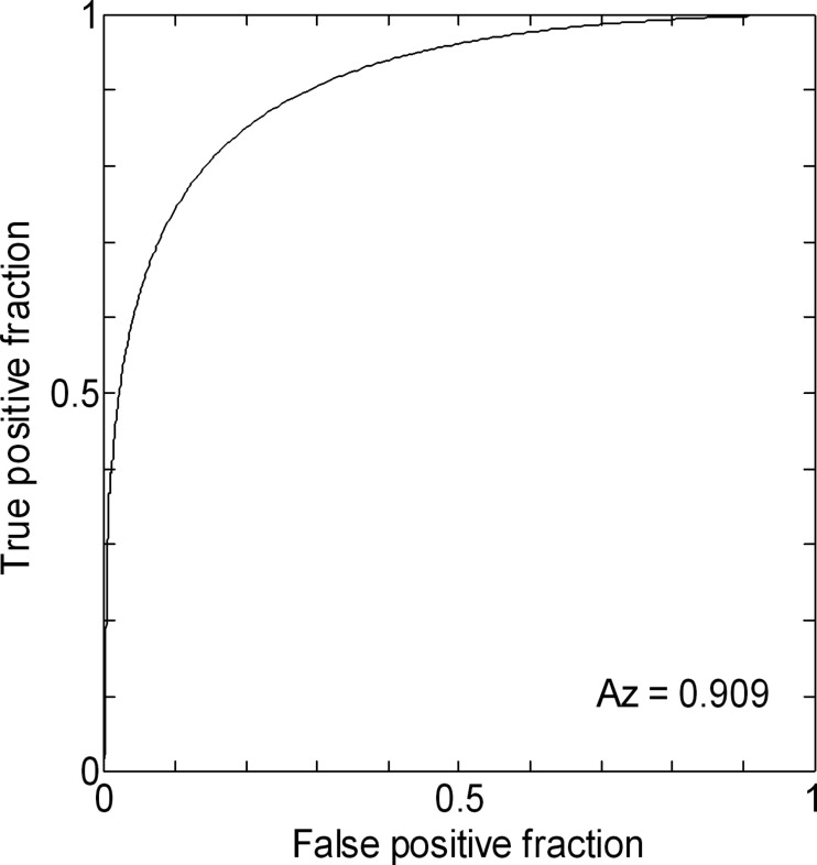
As a result, the area under a receiver operating characteristic (ROC) curve ( Az value) obtained by our computerized method was 0.909 based on a leave-one-out test in identification of AD cases among 54 cases.

Conclusion

This preliminary result showed that our method may be promising for detecting AD patients.

Alzheimer’s disease (AD) is a dementing disorder and one of the major public health problems in countries with greater longevity, such as Japan, where the average citizen lived for 82 years in 2004 ( ). AD is a progressive neurodegenerative disorder of hitherto unknown etiology leading progressively to severe incapacity and death ( ). AD is associated with the atrophy of gray matter in the cerebral cortex, which leads to a volume decrease of the cerebral cortex or a volume increase of cerebrospinal fluid (CSF) in cerebral sulci and lateral ventricles (LVs), which can be measured in magnetic resonance (MR) images. In order to provide appropriate care for AD patients, it is very important to quantitatively evaluate the degree of the atrophy in the cerebral cortex at the early stage of AD. Neuroradiologists attempt to estimate the degree of atrophy by capturing atrophic image features on MR images, but it is very difficult and time consuming in routine clinical practice. Therefore, a number of automated methods for segmentation of gray matter and white matter regions ( ), measurement of the cortical thickness ( ), and volumetric measurement of the CSF in cerebral sulci and LVs ( ) have been studied so that the progression of cerebral atrophy can be monitored. However, such image features have not been employed for identification of AD patients.

In recent years, a whole-brain unbiased objective technique, known as voxel-based morphometry (VBM), has been developed for characterizing differences in the local composition of brain tissue using MR images and can objectively map gray matter loss on a voxel-by-voxel basis ( ). The VBM is achieved by spatially normalizing all brains to the same standardized brain acquired from many normal subjects, segmenting the normalized brain into gray and white matter, smoothing the gray and white matter images, and then finally performing a statistical analysis to localize significant differences between two or more experimental groups. On the other hand, the computer-aided diagnosis (CAD) methods based on a pattern recognition technique using image features have been developed and may be promising for detection of abnormalities in the field of neuroradiology ( ). Therefore, such CAD approaches should be studied for detection of AD patients. To our knowledge, no studies have ever tried to develop CAD systems based on pattern recognition techniques with the atrophic image features, which would be automatically determined. For the purpose, we have developed two automated methods for measurement of the cortical thickness ( ) and for volumetric measurement of CSF regions in cerebral sulci and LVs ( ). In this study, we attempted to develop an automated method for identification of patients with cerebral atrophy due to AD based on a novel pattern recognition technique using 3D MR images.

Materials and methods

Subjects and MRI Data

Get Radiology Tree app to read full this article<

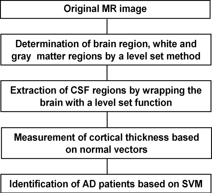
Overall Algorithm

Get Radiology Tree app to read full this article<

Determination of Atrophic Image Features

Volumes of White Matter and Gray Matter Regions

Get Radiology Tree app to read full this article<

ψn+1=ψn−ΔtF∣∣∇ψ∣∣, ψ

−

∇

The new zero level set ψ = 0 moves depending on the speed function F . In this study, the speed function F was given by

F=am(ν−ρκ), F

(

−

)

where

m=11+|∇{Gσ⊗I(x,y,z)}|, m

∇

{

⊗

(

)

}

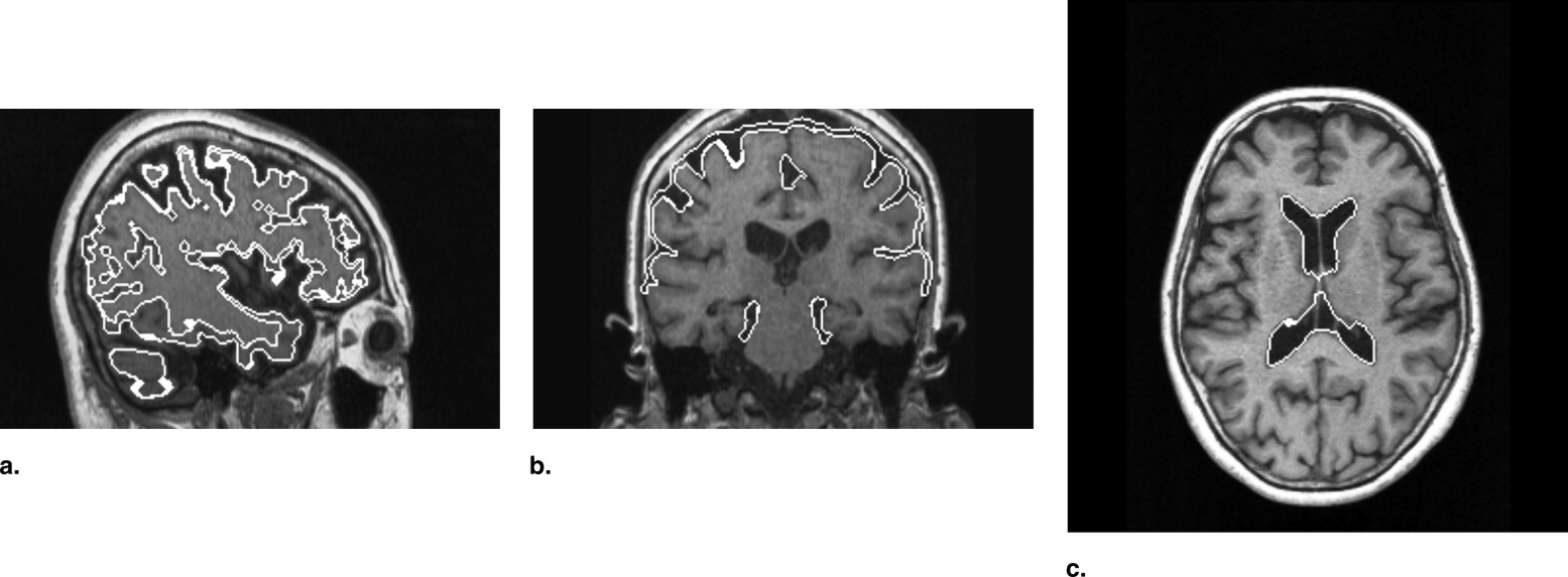
a , ν, and ρ are constants, κ is the mean curvature, G σ is the Gaussian function with a standard deviation of σ , I (x,y,z) is the original image to be processed, and ⊗ means convolution. The constants a and ν function as accelerator and inflation terms, and the curvature κ gives influence on the smoothness of the front. The values a, v, ρ , and σ were set as 1.1, 1.0, 0.5, and 1.1, respectively, which were empirically determined. The value m plays a key role on more accurate segmentation, because the speed function F would decrease and the level set function ψ would hardly change if the moving front approaches an edge of an object. Consequently, we can expect that the zero level set would be at the boundary of a desired object, i.e., the brain surface. Therefore, by monitoring the speed function, the boundary can be determined automatically.

Get Radiology Tree app to read full this article<

Volumes of CSF regions in cerebral sulci and lateral ventricles

Get Radiology Tree app to read full this article<

F=−exp(−α∇{Gσ⊗I(x,y,z)}), F

−

exp

⁡

(

−

∇

{

⊗

(

)

}

)

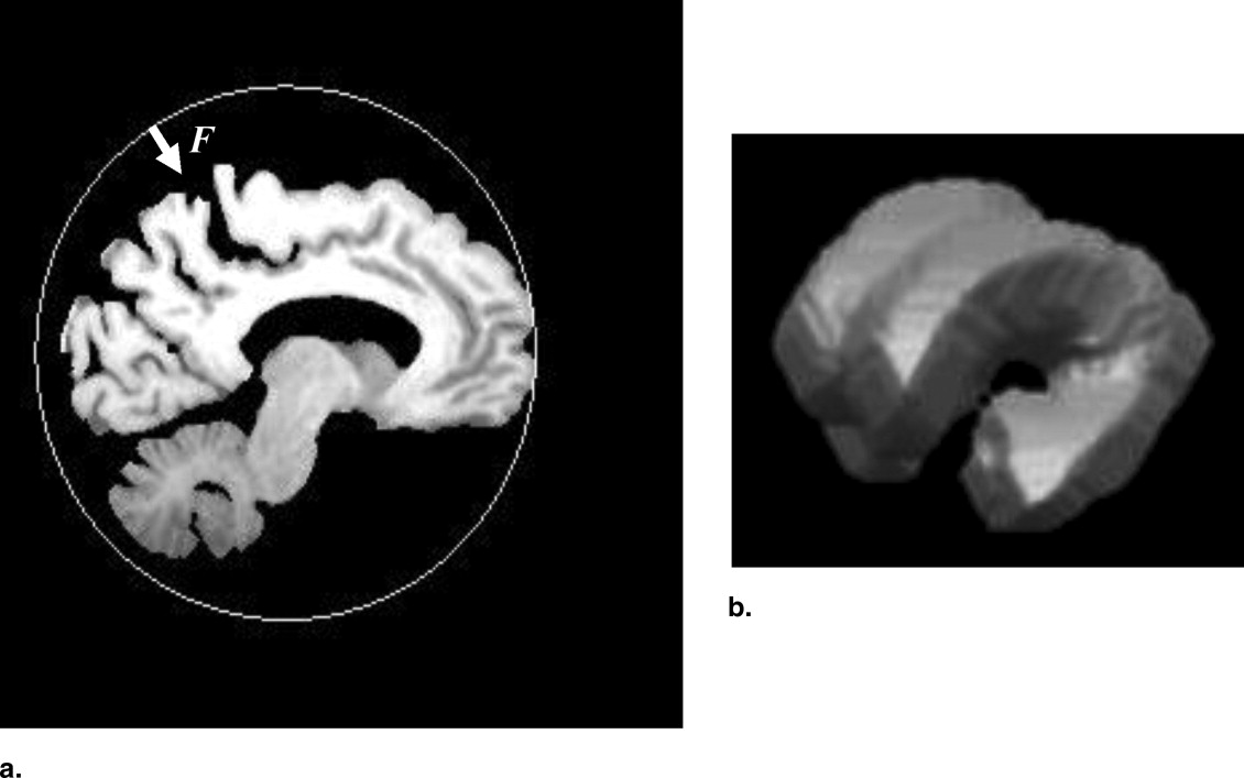
where α is the constant, which was set as α = 3.0 for this study. If the speed F at a center voxel in a region of interest (ROI) with 3 × 3 × 3 would be slower than a threshold speed—i.e., the propagating surface approaches an edge of a brain, the speeds F for 26 neighbors were controlled for wrapping the brain in the propagating surface tightly by the following equation:

Fs=F{1−exp(−βd)}, F

{

−

exp

⁡

(

−

)

}

where Fs is the controlled speed determined by Equation 5 , d is the distance between a voxel and a center of the ROI, and β is the constant, which was set as 0.5 for this study. Consequently, the propagating surface would not intrude sulci and stop at around edge of the brain.

Get Radiology Tree app to read full this article<

Cerebral cortical thickness

Get Radiology Tree app to read full this article<

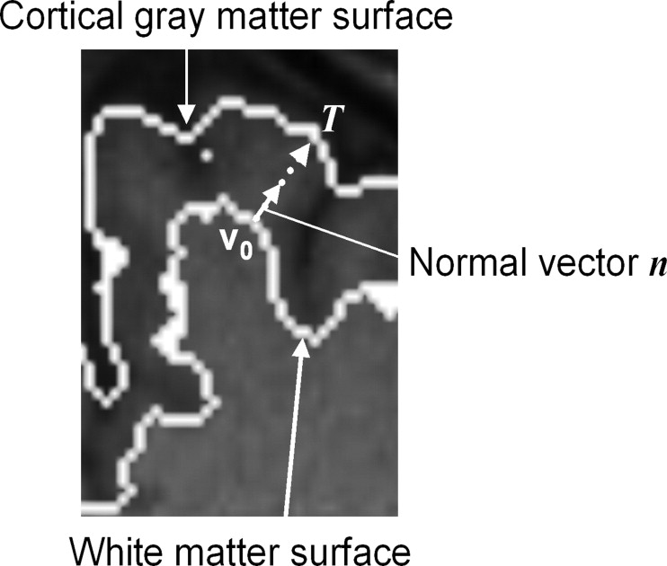
n=∇ψ n

∇

A normal vector for measuring of the cortical thickness is shown by solid line with an arrow in Figure 5 . The cortical thickness was measured from the absolute value of the vector T obtained by extending the normal vector from the white matter surface to the cortical gray matter surface (brain surface) by using the following equation:

T=v0+tn, T

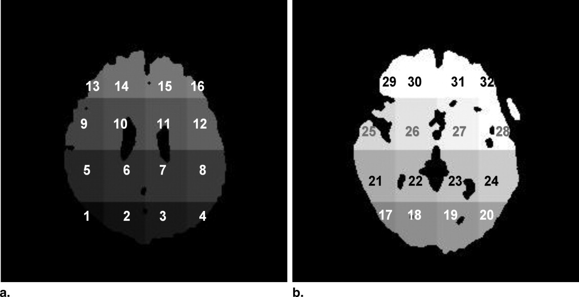
where v 0 is the voxel on the white matter surface and t is the parameter for this linear Equation 7 . Mean cortical thicknesses were measured in the 32 subregions of a brain.

Get Radiology Tree app to read full this article<

Identification of AD Patients Based on Support Vector Machine

Get Radiology Tree app to read full this article<

Get Radiology Tree app to read full this article<

G=∣∣μp−μn∣∣σp+σn, G

−

where μ p and μ n are the mean cortical thicknesses in a subregion for positive (AD) and negative (non-AD) case groups, respectively, and σ p and σ n are the standard deviations of the cortical thicknesses for positive and negative case groups, respectively. Because the Golub statistic can be interpreted as the degree of separation between the two classes, mean cortical thickness in the effective subregion, which indicated Golub statistic greater than a threshold value, was selected for an input of the SVM. In this study, the threshold value was empirically set as 0.6.

Get Radiology Tree app to read full this article<__## Performance Evaluation Method

Get Radiology Tree app to read full this article<__## Results

Get Radiology Tree app to read full this article<

## Discussion

Get Radiology Tree app to read full this article<

## Conclusions

Get Radiology Tree app to read full this article<

## Acknowledgments

Get Radiology Tree app to read full this article<

## Appendix

## Method for Division of a Brain Into Small Subregions

Get Radiology Tree app to read full this article<

## References

- 1. World Health Organization: The World Health Report 2006: Working Together for Health. http://www.who.int/whr/2006/en/index.html

- 2. Jellinger K.A.: Alzheimer 100: Highlights in the history of Alzheimer research. J Neural Transm 2006; 113: pp. 1603-1623.

- 3. Xu C., Pham D.L., Rettmann M.E., et. al.: Reconstruction of the human cerebral cortex from magnetic resonance images. IEEE Trans Med Imaging 1999; 18: pp. 467-480.

- 4. Kovacevic N., Lobaugh N.J., Bronskill M.J., et. al.: A robust method for extraction and automatic segmentation of brain images. NeuroImage 2002; 17: pp. 1087-1100.

- 5. Goldenberg R., Kimmel R., Rivlin E., et. al.: Cortex segmentation: A fast variational geometric approach. IEEE Trans Med Imaging 2002; 21: pp. 1544-1551.

- 6. Zeng X., Staib L.H., Schultz R.T., et. al.: Segmentation and measurement of the cortex from 3D MR images using coupled surfaces propagation. IEEE Trans Med Imaging 1999; 18: pp. 100-101.

- 7. MacDonald D., Kabani N., Avis D., et. al.: Automated 3D extraction of inner and outer surfaces of cerebral cortex from MRI. NeuroImage 2000; 12: pp. 340-356.

- 8. Fischl B., Dale A.M.: Measuring the thickness of the human cerebral cortex from magnetic resonance images. PNAS 2000; 97: pp. 11050-11055.

- 9. Jones S.E., Buchbinder B.R., Aharon I.: Three-dimensional mapping of cortical thickness using Laplace’s equation. Hum Brain Mapp 2000; 11: pp. 12-32.

- 10. Thacker N.A., Varma A.R., Bathgate D.: Dementing disorders: Volumetric measurement of cerebrospinal fluid to distinguish normal from pathologic findings—Feasibility study. Radiology 2002; 224: pp. 278-285.

- 11. Barra V., Frenoux E., Boire J.-Y.: Automatic volumetric measurement of lateral ventricles on magnetic resonance images with correction of partial volume effects. J Magn Reson Imaging 2002; 15: pp. 16-22.

- 12. Ashburner J., Friston K.J.: Voxel-based morphometry: The methods. NeuroImage 2000; 11: pp. 805-821.

- 13. Hirata Y., Matsuda H., Nemoto K., et. al.: Voxel-based morphometry to discriminate early Alzheimer’s disease from controls. Neurosci Lett 2005; 382: pp. 269-274.

- 14. Arimura H., Li Q., Korogi Y., et. al.: Automated computerized scheme for detection of unruptured intracranial aneurysms in three-dimensional MRA. Acad Radiol 2004; 11: pp. 1093-1104.

- 15. Arimura H, Li Q, Korogi Y, et al. Computerized detection of intracranial aneurysms for 3D MR angiography: Feature extraction of small protrusions based on a shape-based difference image technique. Med Phys 33:394–401.

- 16. Arimura H., Yoshiura T., Kumazawa S., et. al.: Computerized method for automated measurement of thickness of cerebral cortex for 3D MR images. SPIE Proc 2006; 6144: pp. 1239-1246.

- 17. Arimura H., Yoshiura T., Kumazawa S., et. al.: Automated volumetric measurement of cerebrospinal fluid in sulci and lateral ventricles based on 3D MR images. IFMBE Proc 2006; 14: pp. 2184-2187.

- 18. Sethian J.A.: Level Set Methods and Fast Marching Methods: Evolving Interfaces in Computational Geometry, Fluid Mechanics, Computer Vision, and Materials Science.1999.Cambridge University PressCambridge

- 19. Malladi R., Sethian J.A., Vemuri B.C.: Shape modeling with front propagation: A level set approach. IEEE Trans Pattern Anal Mach Intell 1995; 17: pp. 158-175.

- 20. Deng J., Tsui H.T.: A fast level set method for segmentation of low contrast noisy biomedical images. Pattern Recogn Lett 2002; 23: pp. 161-169.

- 21. Vapnik V.N.: The Nature of Statistical Learning Theory: Statistics for Engineering and Information Science.2nd ed.1999.Springer-VerlagNew York

- 22. Cristianini N., Shawe-Taylor J.: An Introduction to Support Vector Machines and Other Kernel-Based Learning Methods.2000.Cambridge University PressCambridge

- 23. Joachims T.: _SVM light . Cornell University. http://svmlight.joachims.org/_

- 24. Campadelli P, Casiraghi E, Artioli D. A fully automated method for lung nodule detection from postero-anterior chest radiographs. IEEE Trans Med Imaging 25:1588–1603.

- 25. Golub T.R., Slonim D.K., Tamayo P., et. al.: Molecular classification of cancer: Class discovery and class prediction by gene expression monitoring. Science 1999; 286: pp. 531-537.

- 26. Jain A.K., Duin R.P.W., Jianchang M.: Statistical pattern recognition: a review. IEEE Trans Pattern Anal Mach Intell 2000; 22: pp. 4-37.

- 27. Metz C.E.: ROC Software ROCKIT. http://xray.bsd.uchicago.edu/krl/roc_soft6.htm

- 28. Matsumae M., Kikinis R., Mórocz L., et. al.: Intracranial compartment volumes in patients with enlarged ventricles assessed by magnetic resonance-based image processing. J Neurosurg 1996; 84: pp. 972-981.

- 29. Jorm A.F., Korten E., Henderson A.S.: The prevalence of dementia: A quantitative integration of the literature. Acta Psychiat Scand 1987; 76: pp. 465-479.

- 30. Mölsä P.K., Matilla R.J., Rinne U.K.: Epidemiology of dementia in a Finnish population. Acta Neurol Scand 1982; 65: pp. 541-552.

- 31. Yamada T., Kadekaru H., Matsumoto S., et. al.: Prevalence of dementia in the older Japanese-Brazilian population. Psychiatry Clin Neurosci 2002; 56: pp. 71-75.

Automated Method for Identification of Patients With Alzheimer’s Disease Based on Three-dimensional MR Images

Rationale and Objectives

Materials and Methods

Results

Conclusion

Materials and methods

Subjects and MRI Data

Overall Algorithm

Determination of Atrophic Image Features

Volumes of White Matter and Gray Matter Regions

Volumes of CSF regions in cerebral sulci and lateral ventricles

Cerebral cortical thickness

Identification of AD Patients Based on Support Vector Machine

Further Reading

30% unnecessary

Abstracts of Funded National Institutes of Health Grants

Audience Response Systems in Medical Student Education Benefit Learners and Presenters