Automated Percentage of Breast Density Measurements for Full-field Digital Mammography Applications

Rationale and Objectives

Increased mammographic breast density is a significant risk factor for breast cancer. A reproducible, accurate, and automated breast density measurement is required for full-field digital mammography (FFDM) to support clinical applications. We evaluated a novel automated percentage of breast density measure (PD a ) and made comparisons with the standard operator-assisted measure (PD) using FFDM data.

Methods

We used a nested breast cancer case–control study matched on age, year of mammogram and diagnosis with images acquired from a specific direct x-ray conversion FFDM technology. PD a was applied to the raw and clinical display (or processed) representation images. We evaluated the transformation (pixel mapping) of the raw image, giving a third representation (raw-transformed), to improve the PD a performance using differential evolution optimization. We applied PD to the raw and clinical display images as a standard for measurement comparison. Conditional logistic regression was used to estimate the odd ratios (ORs) for breast cancer with 95% confidence intervals (CI) for all measurements; analyses were adjusted for body mass index. PD a operates by evaluating signal-dependent noise (SDN), captured as local signal variation. Therefore, we characterized the SDN relationship to understand the PD a performance as a function of data representation and investigated a variation analysis of the transformation.

Results

The associations of the quartiles of operator-assisted PD with breast cancer were similar for the raw (OR: 1.00 [ref.]; 1.59 [95% CI, 0.93–2.70]; 1.70 [95% CI, 0.95–3.04]; 2.04 [95% CI, 1.13–3.67]) and clinical display (OR: 1.00 [ref.]; 1.31 [95% CI, 0.79–2.18]; 1.14 [95% CI, 0.65–1.98]; 1.95 [95% CI, 1.09–3.47]) images. PD a could not be assessed on the raw images without preprocessing. However, PD a had similar associations with breast cancer when assessed on 1) raw-transformed (OR: 1.00 [ref.]; 1.27 [95% CI, 0.74–2.19]; 1.86 [95% CI, 1.05–3.28]; 3.00 [95% CI, 1.67–5.38]) and 2) clinical display (OR: 1.00 [ref.]; 1.79 [95% CI, 1.04–3.11]; 1.61 [95% CI, 0.90–2.88]; 2.94 [95% CI, 1.66–5.19]) images. The SDN analysis showed that a nonlinear relationship between the mammographic signal and its variation (ie, the biomarker for the breast density) is required for PD a . Although variability in the transform influenced the respective PD a distribution, it did not affect the measurement’s association with breast cancer.

Conclusions

PD a assessed on either raw-transformed or clinical display images is a valid automated breast density measurement for a specific FFDM technology and compares well against PD. Further work is required for measurement generalization.

Mammographic breast density is a significant breast cancer risk factor . Many of the breast density research studies to date have been based on an operator-assisted measure (PD) to estimate the percentage of breast density within a mammogram. There are various methods under development to automate the estimation of breast density . Developing a fully automated and standardized breast density measurement has proven somewhat difficult, but at least two commercial standardized measures are available for raw full-field digital mammography (FFDM) images: Volpara and Quantra . However, these have not been shown to be associated with breast cancer risk to date.

Although there are various FFDM manufacturers, the two predominant FFDM technologies used today consist of direct and indirect x-ray conversion systems that produce images with different characteristics. The data representation produced by FFDM systems may vary because of the x-ray detection technology, x-ray generation, or postacquisition processing. FFDM systems produce both raw and clinical display (ie, processed) representation mammograms. A given clinical display, or processed image, is derived from its respective raw image with methods developed by the unit’s manufacturer. The raw images are normally not considered in the clinical evaluation. When applying automated methods, it is not clear if both representations result in similar breast density measurements, if there is a preferred representation, or what impact the technology plays.

Get Radiology Tree app to read full this article<

Methods

Study Population and Mammography

Get Radiology Tree app to read full this article<

Statistical Analysis

Get Radiology Tree app to read full this article<

Operator-assisted Percentage of Density

Get Radiology Tree app to read full this article<

Automated Percentage of Breast Density

Get Radiology Tree app to read full this article<

r0i=d1+f1. r

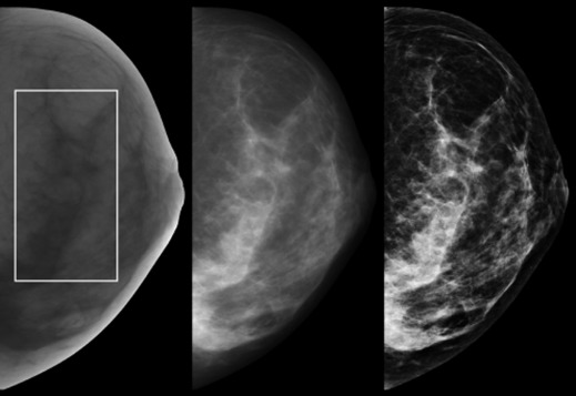
In Equation 1, the subscript, i , defines the three data representations: i = r for raw image, i = t for the raw-transformed image, and i = p for the processed clinical display image. The d 1 and f 1 images are complementary high and low half-band filtered versions (filter outputs) of r 0 i . When the raw image dimension is n x × n y pixels (in the x and y direction), the expansion images have the same dimension.

Get Radiology Tree app to read full this article<

Preprocessing

Get Radiology Tree app to read full this article<

r0t=a0[(m0×r0r)+1]k, r

[

(

)

]

where a 0 and k are parameters determined with the optimization procedure. The pixel values of r 0 r were first linearly mapped between (0, 1) before applying Equation 2 . The m 0 factor is an empirically determined scaling constant ≈101 that constrains the pixel values to the allowable dynamic range and was derived by generalizing the normalization method used in our calibration research work . The m 0 factor is the average current × time (milliampere-second) system readout from a random sample of mammograms. The form of the denominator (addition of one) prevents pixel values in r 0 t from reaching infinity. Equation 2 defines the raw-transformed image representation. We used this 30-image data set to determine these two unknown parameters using an evolutionary optimization strategy .

Get Radiology Tree app to read full this article<

Signal-dependent Noise Analysis

Get Radiology Tree app to read full this article<

y=c0+c1x+c2x2+c3x3+c4exp(−z)2, y

exp

(

−

)

where y is the local noise variance, x is corresponding local signal, z=x−c5c6 z

−

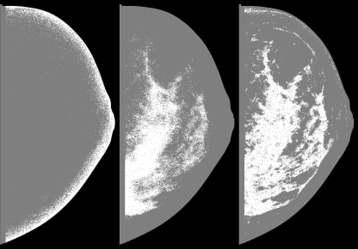
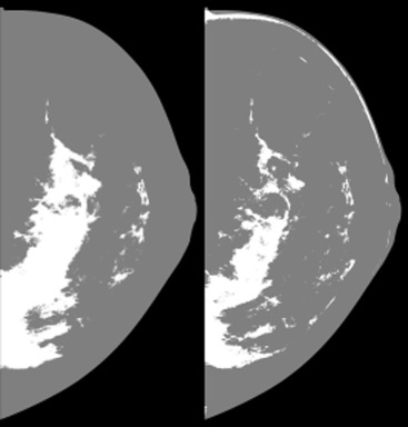
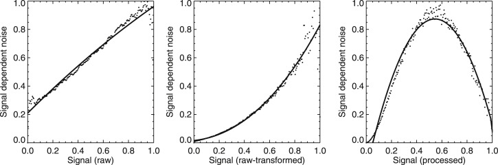
6 , and the c__i are the fit coefficients. Equation 3 is a general expression that was tailored to each representation by initial observation using the 30-image data set discussed previously. For the raw data ( i = r ), we set c 3 = c 4 = c 5 = c 6 = 0; for the raw-transformed data ( i = t ), we set c 4 = c 5 = c 6 = 0; and for the processed data ( i = p ), we set c 3 = 0. Both the signal and noise values were mapped between (0, 1) before applying the curve-fitting analysis. Representative examples are provided to show the differences. We also summarized each representation’s fit-coefficient distributions with the mean (taken over all images) and 95% CIs. For our purpose, c 0 is a bias term used as degree of freedom or flexibility in the fitting processes, and is not discussed in detail.

Get Radiology Tree app to read full this article<

Results

Get Radiology Tree app to read full this article<

Table 1

Patient Characteristics: Distribution of Relevant Patient Characteristics (Variable) and Breast Density Measures for the Cases, Controls, and Overall

Variable Case ( n ) Mean SD Control ( n ) Mean SD Total ( n ) Mean SD_P_ Value Age (years) 192 64.2 10.6 358 64.3 10.6 550 64.3 10.7 — BMI (kg/m 2 ) 188 29.0 6.4 335 28.8 6.2 523 28.9 6.3 .81 PD a (trans) 192 21.0 7.3 358 19.1 7.3 550 19.8 7.4 .002 PD a (proc) 192 19.1 7.9 358 16.9 7.5 550 17.6 7.7 .0005 PD (raw) 192 15.0 12.1 358 13.6 12.5 550 14.1 12.4 .17 PD (proc) 192 18.1 10.3 358 16.9 10.0 550 17.4 10.1 .15

BMI, body mass index.

The breast density measures include 1) the automated percentage of breast density measure (PD a ) applied to the raw-transformed images (trans); 2) PD a applied to the clinical display processed images (proc); 3) operator-assisted percentage of breast density measure (PD) applied to the raw images (raw); and 4) PD applied to the clinical display processed images. The mean and standard deviation (SD) are provided for each characteristic. Breast density quantities are percentages. The respective case–control quantities were compared using conditional logistic regression (Wald test).

Get Radiology Tree app to read full this article<

Table 2

Percentage of Breast Density Associations with Breast Cancer

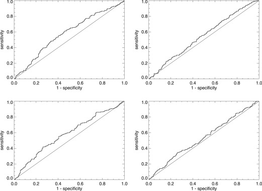
Control ( N ) Case ( N ) Unadjusted Adjusted with BMI PD a raw-transformed Quartile 1 [3.98–13.41] 89 30 1.00 1.00 Quartile 2 [13.41–18.14] 90 40 1.26 (0.73–2.18) 1.27 (0.74–2.19) Quartile 3 [18.14–23.82] 89 50 1.85 (1.05–3.26) 1.86 (1.05–3.28) Quartile 4 [23.82–38.47] 90 72 2.93 (1.64–5.22) 3.00 (1.67–5.38) Az 0.605 (0.569-0.643) 0.606 (0.549-0.654) Per 1 SD increase 1.39 (1.13–1.70) 1.40 (1.14–1.71) Az 0.606 (0.559-0.648) 0.597 (0.550-0.647) PD a processed Quartile 1 [2.99–10.72] 89 27 1.00 1.00 Quartile 2 [10.72–15.80] 90 50 1.80 (1.04–3.12) 1.79 (1.04–3.11) Quartile 3 [15.80–22.14] 89 44 1.61 (0.90–2.88) 1.61 (0.90–2.88) Quartile 4 [22.14–35.37] 90 71 2.89 (1.64–5.09) 2.94 (1.66–5.19) Az 0.602 (0.553-0.647) 0.610 (0.565-0.655) Per 1 SD increase 1.42 (1.16–1.72) 1.43 (1.17–1.74) Az 0.603 (0.560-0.652) 0.600 (0.548-0.649) PD raw Quartile 1 [0.00–4.81] 89 35 1.00 1.00 Quartile 2 [4.81–10.09] 90 50 1.48 (0.88–2.49) 1.59 (0.93–2.70) Quartile 3 [10.09–18.69] 89 49 1.46 (0.85–2.51) 1.70 (0.95–3.04) Quartile 4 [18.69–76.84] 90 58 1.70 (1.00–2.87) 2.04 (1.13–3.67) Az 0.553 (0.520-0.599) 0.575 (0.523-0.624) Per 1 SD increase 1.14 (0.94–1.39) 1.21 (0.97–1.51) Az 0.567 (0.508-0.624) 0.566 (0.507-0.619) PD processed Quartile 1 [1.11–9.63] 89 39 1.00 1.00 Quartile 2 [9.63–15.07] 90 51 1.28 (0.77–2.13) 1.31 (0.79–2.18) Quartile 3 [15.07–21.39] 89 40 1.04 (0.61–1.76) 1.14 (0.65–1.98) Quartile 4 [21.39–67.10] 90 62 1.68 (1.00–2.83) 1.95 (1.09–3.47) Az 0.563 (0.523-0.601) 0.573 (0.526-0.622) Per 1 SD increase 1.15 (0.95–1.38) 1.22 (0.98–1.51) Az 0.551 (0.502-0.599) 0.551 (0.500-0.603)

BMI, body mass index; CI, confidence interval; SD, standard deviation.

This table provides the quartile and continuous breast density associations with breast cancer for 1) the automated measure (PD a ) applied to the raw-transformed ( top left ) and processed clinical display ( bottom left ) representation images and 2) the operator-assisted measure (PD) applied to the raw ( top right ) and processed clinical display ( bottom right ) representations images. Breast density quantities are percentages. Odds ratios are given with 95% CIs parenthetically and the area under the receiver operating characteristic curve (Az) is provided for each model with 95% CIs. Az was calculated within matched case–control pairs to use the design. SD is calculated from the control distribution.

Get Radiology Tree app to read full this article<

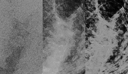
Table 3

Correlation Coefficients

Measurement PD raw PD proc PD a raw-trans PD a proc PD raw 1.00 0.73 0.37 0.46 PD proc 0.73 1.00 0.38 0.43 PD a raw-trans 0.37 0.38 1.00 0.87 PD a proc 0.46 0.43 0.87 1.00

PDa, automated percentage of breast density measure; PD, the operator-assisted measure.

This table lists the inter- and intra-measure Pearson correlation coefficients for PD and PD a . PD was applied to the raw and clinical display processed images (proc), whereas PD a was applied to the raw-transformed (raw-trans) and processed (proc) images.

Table 4

Signal-dependent Noise Model Coefficients

Coefficients Image Representation raw raw-trans proc c 0 0.140 (0.130–0.150) 0.019 (0.017–0.021) −0.111 (−0.116 - −0.106) c 1 0.455 (0.410–0.501) 0.274 (0.255–0.293) 3.001 (2.926–3.076) c 2 0.131 (0.098–0.164) 0.339 (0.265–0.414) −2.265 (−2.390 - −2.141) c 3 — 0.106 (0.047–0.165) — c 4 — — −0.433 (−0.538 - −0.328) c 5 — — 1.038 (1.016–1.060) c 6 — — 0.083 (0.064–0.102)

The table provides the summarized signal-dependent noise modeling coefficients for the three data representations modeled with Equation 3 : raw; raw-transformed (raw-trans); and processed clinical display (proc). For each coefficient, the mean over the entire data set is provided. Confidence intervals are provided with each quantity parenthetically. Terms not included in the modeling are marked with dashes in the respective columns.

Get Radiology Tree app to read full this article<

Discussion

Get Radiology Tree app to read full this article<

Conclusions

Get Radiology Tree app to read full this article<

Acknowledgments

Get Radiology Tree app to read full this article<

Appendix

Repeated Optimization

Get Radiology Tree app to read full this article<

Table 1A

Percentage of Breast Density Associations with Breast Cancer from the Repeated Optimization Trials

PD a Raw Transformed (Min) Control ( N ) Case ( N ) Unadjusted Adjusted with BMI PD a Raw Transformed (Mean) Control ( N ) Case ( N ) Unadjusted Adjusted with BMI PD a Raw Transformed (Max) Control ( N ) Case ( N ) Unadjusted Adjusted with BMI Quartile 1 [1.56–7.25] 89 32 1.00 1.00 Quartile 1 [2.62–10.91] 89 35 1.00 1.00 Quartile 1 [4.06–15.10] 89 35 1.00 1.00 Quartile 2 [7.25–10.94] 90 45 1.42 (0.82–2.46) 1.44 (0.83–2.49) Quartile 2 [10.91–15.61] 90 40 1.13 (0.65–1.98) 1.14 (0.65–2.00) Quartile 2 [15.10–20.85) 90 43 1.19 (0.69–2.06) 1.20 (0.69–2.07) Quartile 3 [10.94–16.08] 89 47 1.52 (0.88–2.64) 1.53 (0.88–2.67) Quartile 3 [15.61–20.79] 89 43 1.29 (0.75–2.24) 1.31 (0.76–2.28) Quartile 3 [20.85–25.02] 89 47 1.36 (0.79–2.34) 1.38 (0.80–2.38) Quartile 4 [16.08–31.94] 90 68 2.45 (1.39–4.32) 2.55 (1.44–4.54) Quartile 4 [20.79–34.42] 90 74 2.35 (1.36–4.06) 2.45 (1.41–4.27) Quartile 4 [25.02–34.98] 90 67 2.05 (1.19–3.54) 2.10 (1.21–3.66) Az 0.58 (0.54–0.63) 0.60 (0.55–0.64) Az 0.59 (0.54–0.63) 0.60 (0.55–0.65) Az 0.59 (0.53–0.62) 0.59 (0.53–0.63) Per 1 SD increase 1.40 (1.15–1.72) 1.44 (1.17–1.77) Per 1 SD increase 1.37 (1.12–1.67) 1.39 (1.13–1.70) Per 1 SD increase 1.26 (1.03–1.53) 1.27 (1.04–1.55) Az 0.62 (0.57–0.66) 0.60 (0.56–0.65) Az 0.60 (0.55–0.64) 0.59 (0.55–0.65) Az 0.59 (0.53–0.64) 0.60 (0.54–0.64)

BMI, body mass index; CI, confidence interval; SD, standard deviation.

This table provides the breast cancer quartile and continuous breast density associations with breast cancer for the automated measure (PDa) applied to the raw-transformed data using the parameter set with the minimum value of k (Min) on the left , parameter set comprised of the distribution averages of both parameters ( middle ), and the set containing the maximum value of k (Max) on the right . Breast density quantities are percentages. Odds ratios are given with 95% CIs parenthetically, and the area under the receiver operating characteristic curve (Az) is provided for each model with 95% CIs. Az was calculated within matched case–control pairs to use the design. SD is calculated from the control distribution.

Get Radiology Tree app to read full this article<

References

1. Boyd N.F., Guo H., Martin L.J., et. al.: Mammographic density and the risk and detection of breast cancer. N Engl J Med 2007; 356: pp. 227-236.
2. McCormack V.A., dos Santos Silva I.: Breast density and parenchymal patterns as markers of breast cancer risk: a meta-analysis. Cancer Epidemiol Biomarkers Prev 2006; 15: pp. 1159-1169.
3. Boyd N.F., Martin L.J., Yaffe M.J., et. al.: Mammographic density and breast cancer risk: current understanding and future prospects. Breast Cancer Res 2011; 13: pp. 223.
4. Yaffe M.J.: Mammographic density. Measurement of mammographic density. Breast Cancer Res 2008; 10: pp. 209.
5. Keller B.M., Nathan D.L., Wang Y., et. al.: Estimation of breast percent density in raw and processed full field digital mammography images via adaptive fuzzy c-means clustering and support vector machine segmentation. Med Phys 2012; 39: pp. 4903-4917.
6. Manduca A., Carston M.J., Heine J.J., et. al.: Texture features from mammographic images and risk of breast cancer. Cancer Epidemiol Biomarkers Prev 2009; 18: pp. 837-845.
7. Highnam R., Brady M.: Mammographic image analysis.1999.Kluwer Academic PublishersBoston, MA
8. Pawluczyk O., Augustine B.J., Yaffe M.J., et. al.: A volumetric method for estimation of breast density on digitized screen-film mammograms. Med Phys 2003; 30: pp. 352-364.
9. Shepherd J.A., Herve L., Landau J., et. al.: Novel use of single X-ray absorptiometry for measuring breast density. Technol Cancer Res Treat 2005; 4: pp. 173-182.
10. Tice J.A., Cummings S.R., Ziv E., et. al.: Mammographic breast density and the Gail model for breast cancer risk prediction in a screening population. Breast Cancer Res Treat 2005; 94: pp. 115-122.
11. Highnam R., Pan X., Warren R., et. al.: Breast composition measurements using retrospective standard mammogram form (SMF). Phys Med Biol 2006; 51: pp. 2695-2713.
12. Jeffreys M., Warren R., Highnam R., et. al.: Initial experiences of using an automated volumetric measure of breast density: the standard mammogram format. Br J Radiol 2006; 79: pp. 378-382.
13. Heine J.J., Thomas J.A.: Effective x-ray attenuation coefficient measurements from two full field digital mammography systems for data calibration applications. Biomed Eng Online 2008; 7: pp. 13.
14. Jeffreys M., Warren R., Highnam R., et. al.: Breast cancer risk factors and a novel measure of volumetric breast density: cross-sectional study. Br J Cancer 2008; 98: pp. 210-216.
15. Heine J.J., Cao K., Beam C.: Cumulative sum quality control for calibrated breast density measurements. Med Phys 2009; 36: pp. 5380-5390.
16. Malkov S., Wang J., Kerlikowske K., et. al.: Single x-ray absorptiometry method for the quantitative mammographic measure of fibroglandular tissue volume. Med Phys 2009; 36: pp. 5525-5536.
17. Boyd N., Martin L., Gunasekara A., et. al.: Mammographic density and breast cancer risk: evaluation of a novel method of measuring breast tissue volumes. Cancer Epidemiol Biomarkers Prev 2009; 18: pp. 1754-1762.
18. Heine J.J., Cao K., Thomas J.A.: Effective radiation attenuation calibration for breast density: compression thickness influences and correction. Biomed Eng Online 2010; 9: pp. 73.
19. Highnam R., Brady M., Yaffe M.J., et. al.: Robust breast composition measurement–Volpara TM .Marti J.IWDM 2010.2010.Springer-Verlagpp. 342-349.
20. Shepherd J.A., Kerlikowske K., Ma L., et. al.: Volume of mammographic density and risk of breast cancer. Cancer Epidemiol Biomarkers Prev 2011; 20: pp. 1473-1482.
21. Ciatto S., Bernardi D., Calabrese M., et. al.: A first evaluation of breast radiological density assessment by QUANTRA software as compared to visual classification. Breast 2012; 21: pp. 503-506.
22. Highnam R., Sauber N., Destounis S., et. al.: Breast density into clinical practice.Maidment A.D.A.Bakic P.R.Gavenonis S.11th International Workshop of Digital Mammography.2012.SpringerPhiladelphia, PA:pp. 466-473.
23. Skippage P., Wilkinson L., Allen S., et. al.: Correlation of age and HRT use with breast density as assessed by Quantra. The Breast Journal 2013; 19: pp. 79-86.
24. Bick U., Diekmann F.: Medical radiology diagnostic imaging and radiation oncology.Baert A.L.Brady L.W.Heilmann H.-P. et. al.Continuation of Handbuch der medizinischen Radiologie Encyclopedia of Medical Radiology.2010.Springer-VerlagBerlin:
25. Kim H.K., Cunningham I.A., Yin Z., et. al.: On the development of digital radiography detectors: A review. Int J Precis Eng Man 2008; 9: pp. 86-100.
26. Mahesh M.: AAPM/RSNA physics tutorial for residents: digital mammography: an overview. Radiographics 2004; 24: pp. 1747-1760.
27. Heine J.J., Deans S.R., Velthuizen R.P., et. al.: On the statistical nature of mammograms. Med Phys 1999; 26: pp. 2254-2265.
28. Heine J.J., Velthuizen R.P.: A statistical methodology for mammographic density detection. Med Phys 2000; 27: pp. 2644-2651.
29. Heine J.J., Carston M.J., Scott C.G., et. al.: An automated approach for estimation of breast density. Cancer Epidemiol Biomarkers Prev 2008; 17: pp. 3090-3097.
30. Heine J.J., Behera M.: Aspects of signal-dependent noise characterization. J Opt Soc Am A 2006; 23: pp. 806-815.
31. Olson J.E., Sellers T.A., Scott C.G., et. al.: The influence of mammogram acquisition on the mammographic density and breast cancer association in the mayo mammography health study cohort. Breast Cancer Res 2012; 14: pp. R147.
32. Heine J.J., Scott C.G., Sellers T.A., et. al.: A novel automated mammographic density measure and breast cancer risk. Journal of the National Cancer Institute 2012; 104: pp. 1028-1037.
33. Hosmer D.W., Lemeshow S.: Applied logistic regression.Second Edition2000.John Wiley & Sons IncHoboken
34. Breslow N., Day N.: The analysis of case-control studies. IARC Sci Publ 1980; 32: pp. 147-178.
35. Vachon C.M., Fowler E.E., Tiffenberg G., et. al.: Comparison of percent density from raw and processed full-field digital mammography data. Breast Cancer Res 2013; 15: pp. R1.
36. Heine J.J., Deans S.R., Cullers D.K., et. al.: Multiresolution statistical analysis of high-resolution digital mammograms. IEEE Trans Med Imaging 1997; 16: pp. 503-515.
37. Heine J.J., Deans S.R., Cullers D.K., et. al.: Multiresolution probability analysis of gray-scaled images. J Opt Soc Am A 1998; 15: pp. 1048-1058.
38. Heine J.J., Deans S.R., Gangadharan D., et. al.: Multiresolution analysis of two-dimensional 1/f processes: approximation methods for random variable transformations. OPT ENG 1999; 38: pp. 1505.
39. Fowler E.E., Lu B., Heine J.J.: A comparison of calibration data from full field digital mammography units for breast density measurements. Biomed Eng Online 2013; 12: pp. 114.
40. Price K.V., Storn R.M., Lampinen J.A.: Differential evolution: a practical approach to global optimization.2005.SpringerBerlin ; New York
41. Behera M., Fowler E.E., Owonikoko T.K., et. al.: Statistical learning methods as a preprocessing step for survival analysis: evaluation of concept using lung cancer data. Biomed Eng Online 2011; 10: pp. 97.
42. Heine J.J., Cao K., Rollison D.E., et. al.: A quantitative description of the percentage of breast density measurement using full-field digital mammography. Acad Radiol 2011; 18: pp. 556-564.
43. Heine J.J., Cao K., Rollison D.E.: Calibrated measures for breast density estimation. Acad Radiol 2011; 18: pp. 547-555.
44. Fowler E.E., Sellers T.A., Lu B., et. al.: Breast Imaging Reporting and Data System (BI-RADS) breast composition descriptors: automated measurement development for full field digital mammography. Med Phys 2013; 40: pp. 113502.
45. Keller B.M., Nathan D.L., Gavenonis S.C., et. al.: Reader variability in breast density estimation from full-field digital mammograms: the effect of image postprocessing on relative and absolute measures. Acad Radiol 2013; 20: pp. 560-568.
46. Griffin W.C.: Transform techniques for probability modeling.1975.Academic PressNew York
47. Ding J., Warren R., Warsi I., et. al.: Evaluating the effectiveness of using standard mammogram form to predict breast cancer risk: case-control study. Cancer Epidemiol Biomarkers Prev 2008; 17: pp. 1074-1081.
48. Heine J.J., Fowler E.E., Flowers C.I.: Full field digital mammography and breast density: comparison of calibrated and noncalibrated measurements. Acad Radiol 2011; 18: pp. 1430-1436.
49. Schousboe J.T., Kerlikowske K., Loh A., et. al.: Personalizing Acad Radiol mammography by breast density and other risk factors for breast cancer: analysis of health benefits and cost-effectiveness. Annals of internal medicine 2011; 155: pp. 10-20.
50. FDA. MQSA National statistics. Available at: http://www.fda.gov/Radiation-EmittingProducts/MammographyQualityStandardsActandProgram/FacilityScorecard/ucm113858.htm .
51. MarketRseacrh.com. Full-field digital mammography equipment–Global Pipeline Analysis, Competitive Landscape and Market Forecasts to 2017. Available at: F:∖Full-Field Digital Mammography Equipment - Global Pipeline Analysis, Competitive Landscape and Market Forecasts to 2017 by GlobalData in Mammography.mht .

Automated Percentage of Breast Density Measurements for Full-field Digital Mammography Applications

Rationale and Objectives

Methods

Results

Conclusions

Methods

Study Population and Mammography

Statistical Analysis

Operator-assisted Percentage of Density

Automated Percentage of Breast Density

Preprocessing

Signal-dependent Noise Analysis

Results

Discussion

Conclusions

Acknowledgments

Appendix

Repeated Optimization

References

Further Reading

A Multiobserver Study of the Effects of Including Point-of-care Patient Photographs with Portable Radiography

A Workflow to Improve the Alignment of Prostate Imaging with Whole-mount Histopathology

Dual-energy KUB Radiographic Examination for the Detection of Renal Calculus