Automated Segmentation of the Liver from 3D CT Images Using Probabilistic Atlas and Multilevel Statistical Shape Model

Rationale and Objectives

An atlas-based automated liver segmentation method from three-dimensional computed tomographic (3D CT) images has been developed. The method uses two types of atlases, a probabilistic atlas (PA) and a statistical shape model (SSM).

Materials and Methods

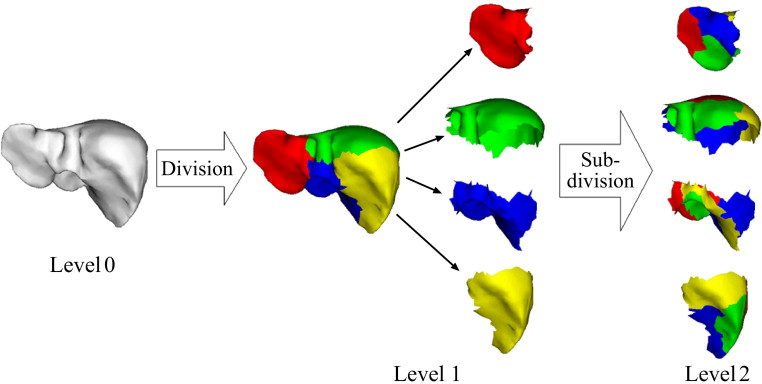
Voxel-based segmentation with a PA is first performed to obtain a liver region, then the obtained region is used as the initial region for subsequent SSM fitting to 3D CT images. To improve reconstruction accuracy, particularly for highly deformed livers, we use a multilevel SSM (ML-SSM). In ML-SSM, the entire shape is divided into patches, with principal component analysis applied to each patch. To avoid inconsistency among patches, we introduce a new constraint called the “adhesiveness constraint” for overlapping regions among patches.

Results

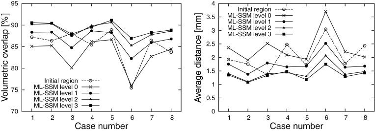
The PA and ML-SSM were constructed from 20 training datasets. We applied the proposed method to eight evaluation datasets. On average, volumetric overlap of 89.2 ± 1.4% and average distance of 1.36 ± 0.19 mm were obtained.

Conclusions

The proposed method was shown to improve segmentation accuracy for datasets including highly deformed livers. We demonstrated that segmentation accuracy is improved using the initial region obtained with PA and the introduced constraint for ML-SSM.

Segmentation of the liver from three-dimensional (3D) data is a prerequisite for computer-assisted diagnosis and preoperative planning. Prior information on the liver, typically represented as a statistical atlas, is useful for robust segmentation. Two types of statistical atlases, the statistical shape model (SSM) ( ) and the probabilistic atlas (PA) ( ), have been used to increase the robustness of segmentation.

An SSM is widely used for organ segmentation and the potential performance for liver segmentation has been shown ( ). However, previous methods using SSM experienced the following problems: 1) an essential limitation to reconstruction accuracy, particularly for diseased livers involving large deformations and lesions; and 2) good initialization is required to obtain proper convergence. One approach to overcome the first problem is to use a multilevel SSM (ML-SSM) ( ), in which the entire organ shape is divided into multiple patches, which are further subdivided at finer representation levels. One problem with ML-SSM, however, is inconsistency among patches at finer levels. Attempts have been made to solve this inconsistency problem ( ), but not for the liver, which displays a highly complex shape and large interpatient variability. Another approach to addressing the first problem is to perform SSM fitting followed by shape-constrained deformable model fitting ( ). However, shape constraints inherent in the liver are not embedded in the deformable model, and robustness against large deformations and lesions has not been verified. Furthermore, the second problem has not been addressed in previous studies. Heimann et al reported that not a few cases failed to converge because of the initialization problem ( ).

Get Radiology Tree app to read full this article<

Materials and methods

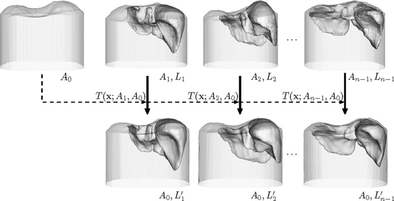
Spatial Normalization Using the Abdominal Cavity

Get Radiology Tree app to read full this article<

Li′={x+t(x;Ai,Ao)|x∈Li}. L

′

{

(

;

)

∈

}

Get Radiology Tree app to read full this article<

Establishing Correspondences of the Liver for Constructing ML-SSM

Get Radiology Tree app to read full this article<

Mi={x+t(x;L0,Li′)|x∈L0}(i=1,⋅⋅⋅,n−1). M

{

(

;

′

)

∈

}

(

⋅

−

)

Get Radiology Tree app to read full this article<

3 Get Radiology Tree app to read full this article<

M¯¯¯¯=1n∑n−1i=0Mi M

∑

−

where M 0 = L 0 . Get Radiology Tree app to read full this article<

4 Get Radiology Tree app to read full this article<

Mi′={x+t(x;M¯¯¯¯,Li′)∣∣x∈M¯¯¯¯}(i=0,1,⋅⋅⋅,n−1). M

′

{

(

;

′

)

∈

}

(

⋅

−

)

Get Radiology Tree app to read full this article<

Using the above procedure, Mi′(i=0,1,⋅⋅⋅,n−1) M

′

(

⋅

−

) was obtained, where surface points corresponded among the different liver shapes.

Get Radiology Tree app to read full this article<

Constructing Statistical Atlases

Get Radiology Tree app to read full this article<

P(x)=1n∑n−1i=0Bi(x). P

(

)

∑

−

(

)

Get Radiology Tree app to read full this article<

Constructing a ML-SSM

Get Radiology Tree app to read full this article<

qℓj(bℓj)=q¯ℓj+Φℓjbℓj(j=1,⋅⋅⋅,Nℓ) q

ℓ

(

ℓ

)

ℓ

(

⋅

ℓ

)

where Ф ℓj is the matrix of eigenvectors { uℓj k } and bℓj is the shape parameter vector of the j -th patch at level ℓ .

Get Radiology Tree app to read full this article<

Segmentation of the Liver Using Statistical Atlases

Get Radiology Tree app to read full this article<

b Get Radiology Tree app to read full this article<

Get Radiology Tree app to read full this article<

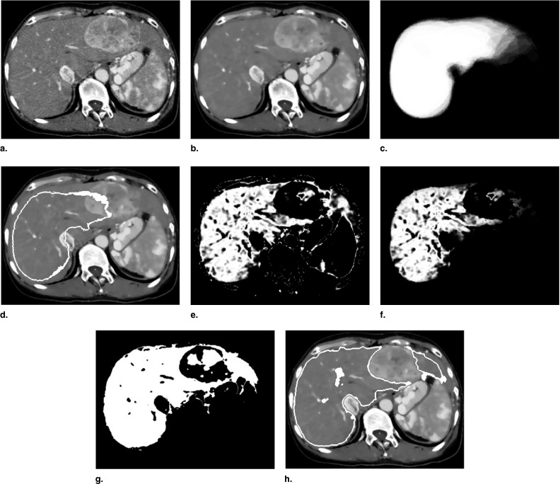
Initial Region Extraction Using Voxel-based Segmentation with PA

Get Radiology Tree app to read full this article<

Q(x)=exp(−(I(x)−I¯)22σ2) Q

(

)

⁡

(

−

(

)

−

)

where Ī and σ represent average intensity and standard deviation, respectively, as estimated based on histographic analysis inside the volume of interest ( ). Q ( x ) is defined as the Gaussian of I ( x ) and is largest when I ( x ) is the same as the average intensity Ī . Given Q ( x ) and P ( x ), the combined likelihood image Q ′( x ) ( Fig 3 f) is defined as

Q′(x)=Q(x)P(x). Q

′

(

)

(

)

(

)

Note that the voxel values of Q ′( x ) are normalized between 0 and 1. The binary image is extracted by thresholding Q ′( x ) using a fixed threshold value T likelihood ( Fig 3 g). The initial region is extracted by opening and closing the binary image ( Fig 3 h).

Get Radiology Tree app to read full this article<

Estimation of Initial Shape Parameters

Get Radiology Tree app to read full this article<

CD(q0(b0);R)=1|q0(b0)|∑x∈q0(b0)w(d(x,R))d(x,R)2+1|R|∑x∈Rw(d(x,q0(b0)))d(x,q0(b0))2 C

(

)

;

)

(

)

∑

∈

(

)

(

)

(

)

∑

∈

(

)

(

)

where d ( x , S ) is the Euclidean distance between point x and surface S , and | · | denotes the number of vertices of the surface model. Robust weight function w ( x ) is used to deal with outliers because of large lesions ( ). w ( x ) is defined as

w(x)={1s|x|ifif|x||x|≤s>s w

(

)

{

≤

where s is the robust standard deviation given by s = max (1.4826 × median{| d k − median( d k )|}, 5.0 mm), and d__k is the residual in millimeters at each vertex of q 0 (b 0 ). The Levenberg-Marquardt algorithm is used to minimize Equation 9 . The average shape, that is, b 0 = 0 , is used for the initial parameter of the minimization.

Get Radiology Tree app to read full this article<

Segmentation Processes Using ML-SSM

Get Radiology Tree app to read full this article<

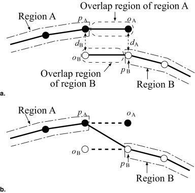
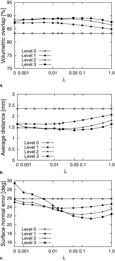
C(qℓ(bℓ);P)=CD(qℓ(bℓ);P)+λCA(qℓ(bℓ)) C

(

ℓ

(

ℓ

)

;

)

(

ℓ

(

ℓ

)

;

)

(

ℓ

(

ℓ

)

where C D ( q ℓ ( bℓ ); P ) is the sum of distances between the model surface qℓ and edge points P , and C A ( qℓ ( bℓ )) is the adhesiveness constraint for overlap regions to eliminate inconsistency among adjacent patches. Furthermore, λ is a weight parameter balancing the two constraints. λ was determined experimentally. Figure 4 a shows the definition of the adhesiveness constraint as a two-dimensional schematic diagram. Black and white nodes indicate the vertices of regions A and B, respectively, and solid lines denote polygons of surface models. Let pA and pB denote the vertices on the boundaries of regions A and B, respectively. Let oA and oB denote the overlap regions of regions A and B, respectively. Let d__A be the distance between oA and corresponding vertex pB of the adjacent region B. Let d__B be the distance between oB and corresponding vertex pA of the adjacent region A. The adhesiveness constraint avoids increasing these distances d__A and d__B . Cost functions of the sum of distances C D ( q ℓ ( bℓ ); P ) and the adhesiveness constraint C A ( q ℓ ( bℓ )) are defined as

CD(qℓ(bℓ);P)=1|qℓ(bℓ)|∑x∈qℓ(bℓ)w(miny∈P∥x−y∥∥∥)miny∈P∥x−y∥2+1|P|∑x∈Pw(d(x,qℓ(bℓ)))d(x,qℓ(bℓ))2 C

(

ℓ

(

ℓ

)

;

)

ℓ

(

ℓ

)

∑

∈

ℓ

(

ℓ

)

(

⁡

∈

∥

−

∥

)

⁡

∈

∥

−

∥

∑

∈

(

ℓ

(

ℓ

)

(

ℓ

(

ℓ

)

CA(qℓ(bℓ))=1∑Nℓj=1|Oℓj|∑Nℓj=1∑x∈Oℓj(x−x′)2 C

(

ℓ

(

ℓ

)

∑

ℓ

∑

ℓ

∑

∈

ℓ

(

−

′

)

where || v || is the norm of vector v , O__ℓj is the overlap region of the j -th patch at level ℓ and x ′ is the point that corresponds to x in the overlap region of the adjacent patch ( pA and pB corresponding to oB and oA , respectively, in Figure 4 a.

Get Radiology Tree app to read full this article<

Results

Experimental Conditions

Get Radiology Tree app to read full this article<

Experimental Results

Get Radiology Tree app to read full this article<

Table 1

Evaluation of Segmentation Accuracy

Initialization Using Segmentation with PA Using Segmentation with PA Using Average Shape Using Average Shape Adhesiveness Constraint λ = 0 λ = 0.05 λ = 0 λ = 0.05 Initial region 85.2/2.06 85.2/2.06 −/− −/− Level 0 83.3/2.34 83.3/2.34 81.1/3.12 81.1/3.12 Level 1 87.2/1.65 86.7/1.76 84.3/2.53 84.0/2.69 Level 2 88.4/1.47 88.7/1.45 85.1/2.28 86.0/2.34 Level 3 87.5/1.6489.2/1.36 84.9/2.34 86.4/2.20

PA, probabilistic atlas.

Volumetric overlap (%)/average symmetric absolute surface distance (mm).

Averages of eight datasets of volumetric overlap (percentage) and average symmetric absolute surface distance (millimeters) (divided by slash) are shown for each experimental condition. The results of the proposed method are enhanced.

Get Radiology Tree app to read full this article<

Discussion

Get Radiology Tree app to read full this article<

Conclusion

Get Radiology Tree app to read full this article<

References

1. Cootes T.F., Taylor C.J., Cooper D.H., et. al.: Active shape models—their training and application. Comp Vision Image Understanding 1995; 61: pp. 38-59.
2. Leventon M.E., Grimson W.E.L., Faugeras O.: Statistical shape influence in geodesic active contours. Proc IEEE Computer Soc Conf Computer Vision Pattern Recognition 2000; 1: pp. 316-323.
3. Bailleul J., Ruan S., Constans J.M.: Statistical shape model-based segmentation of brain MRI images. 29th Annual International Conference of IEEE-EMBS, Engineering in Medicine and Biology Society, No. 43535272007.Cité InternationaleLyon, France:pp. 5255-5258.
4. Shen D., Herskovits E.H., Davatzikos C.: An adaptive-focus statistical shape model for segmentation and shape modeling of 3-D brain. IEEE Trans Med Imaging 2001; 20: pp. 257-270.
5. Park H., Bland P.H., Meyer C.R.: Construction of an abdominal probabilistic atlas and its application in segmentation. IEEE Trans Med Imaging 2003; 22: pp. 483-492.
6. Joshi S., Davis B., Jomier M., et. al.: Unbiased diffeomorphic atlas construction for computational anatomy. NeuroImage 2004; 23: pp. S151-S160.
7. Straka M., Cruz A.L., Dimitrov L., et. al.: Bone segmentation in CT-angiography data using a probabilistic atlas. Vision Modeling Visualization 2003; pp. 505-512.
8. Lamecker H., Lange T., Seebaβ M.: Segmentation of the liver using a 3D statistical shape model.2004.Technical report, Zuse InstitueBerlin
9. Heimann T., Wolf I., Meinzer H.P.: Active shape models for a fully automated 3D segmentation of the liver— an evaluation on clinical data.2006. Lect Notes Computer Sci 4191 (Proc MICCAI 2006, Part II), Copenhagen, Denmark; 41–48.
10. Davatzikos C., Tao X., Shen D.: Hierarchical active shape models, using the wavelet transform. IEEE Trans Med Imaging 2003; 22: pp. 414-423.
11. Zhao Z., Aylward S.R., Teoh E.K.: A novel 3D partitioned active shape model for segmentation of brain MR images.2005. Lect Notes Computer Sci; 3749 (Proc MICCAI 2005, Part I), Palm Springs, CA, 221–228.
12. Yokota K., Okada T., Nakamoto M., et. al.: Construction of conditional statistical atlases of the liver based on spatial normalization using surrounding structures.2006. Proc Computer Assisted Radiol Surg (CARS 2006), Osaka, Japan; 39–40.
13. Zhou X., Kitagawa T., Hara T., et. al.: Constructing a probabilistic model for automated liver region segmentation using non-contrast x-ray torso CT images.2006. Lect Notes Computer Sci; 4191 (Proc MICCAI 2006, Part II), Copenhagen, Denmark, 856–863.
14. Okada T., Shimada R., Sato Y., et. al.: Automated segmentation of the liver from 3D CT images using probabilistic atlas and multi-level statistical shape model.2007. Lect Notes Computer Sci; 4791 (Proc MICCAI 2007, Part I), Brisbane, Australia:86–93.
15. Chui H., Rangarajan A.: A new point matching algorithm for non-rigid registration. Computer Visi Image Understanding 2003; 89: pp. 114-141.
16. Besl P.J., Birch J.B., Watson L.T.: Robust window operators. Machine Vis Appl 1989; 2: pp. 179-191.
17. Garland M., Heckbert P.: Surface simplification using quadric error metrics. SIGGRAPH ‘97 1997; pp. 209-216.
18. Heimann T., van Ginneken B., Styner M.: MICCAI workshop on 3D segmentation in the clinic. http://mbi.dkfz-heidelberg.de/grand-challenge2007/ Accessed March 17, 2008.
19. Okada T., Yokota K., Nakamoto M., et. al.: Multi-level statistical shape model using shape stabilization terms for generic modeling of organs. Trans Inst Electron Inform Commun Eng D J91-D 2008; pp. 1862-1873. [in Japanese].
20. Couinaud C.: The paracaval segments of the liver. J Hepato Bil Pancr Surg 1994; 1: pp. 145-151.

Automated Segmentation of the Liver from 3D CT Images Using Probabilistic Atlas and Multilevel Statistical Shape Model

Rationale and Objectives

Materials and Methods

Results

Conclusions

Materials and methods

Spatial Normalization Using the Abdominal Cavity

Establishing Correspondences of the Liver for Constructing ML-SSM

Constructing Statistical Atlases

Constructing a ML-SSM

Segmentation of the Liver Using Statistical Atlases

Initial Region Extraction Using Voxel-based Segmentation with PA

Estimation of Initial Shape Parameters

Segmentation Processes Using ML-SSM

Results

Experimental Conditions

Experimental Results

Discussion

Conclusion

References

Further Reading

Abstracts of Funded National Institutes of Health Grants

Advances in Radiological Image Analysis from MICCAI 2007

Automated 11 C-PiB Standardized Uptake Value Ratio