Automatic and Rapid Identification of Infarct Slices and Hemisphere in DWI Scans

Rationale and Objectives

Accurate, free of observer’s bias, and fast identification of acute infarct is critical in visual and automatic processing of stroke images. An automatic and rapid algorithm has been developed to identify the infarct slices and the hemisphere in diffusion-weighted imaging (DWI) scans.

Materials and Methods

Thirty-six DWI scans were acquired from five centers with the slice thickness of 4–14 mm. We also derive images from the original scans to assess the accuracy of the algorithm by using a wide range of infarct size and number of artifacts per unit area. Based on the difference in percentile characteristics of intensity normalized (infarct/noninfarct) images, two parameters are defined: R s for infarct slice identification and R h for infarct hemisphere identification. Using the identified infarct slices the infarct hemisphere is subsequently determined.

Results

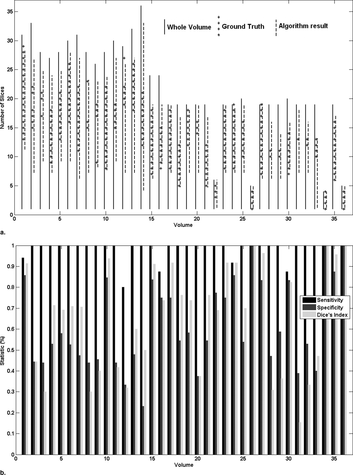
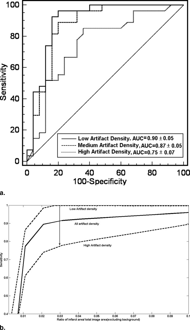
The average sensitivity and specificity for slice and hemisphere identification were 98.1%, 51.4% and 91.7%, 91.7%, respectively. The processing time is ∼3–5 seconds on Matlab platform and on VC++ it is predicted ∼10 milliseconds. Based on simulation study, we can infer that the algorithm produces accurate results in most of the situations although the sensitivity goes down by ∼15% when the infarct size is small (<2–3% of image area) and the artifacts per unit area are large.

Conclusions

The proposed algorithm applied as a preprocessor can be useful to: 1) estimate location (hemisphere) and extent of infarct (number and location of slices), 2) reduce time and labor of infarct volume study, 3) cross-check visual interpretation, 4) form a part of an infarct segmentation module, and 5) improve localization of the midsagittal plane.

Diffusion-weighted Imaging (DWI) is used to evaluate infarct in acute ischemic stroke patients. Automatic and rapid identification of infarcts in DWI images is important both in visual scan reading and automatic image processing as it reduces time and increases confidence. More importantly, as a recent study ( ) shows, infarct location is fundamentally linked to neurologic deficits. Several automatic or semiautomatic segmentation techniques are proposed to reduce the total time of infarct segmentation compared with manual processing of data, which may have errors and observer’s bias. A semiautomatic method ( ) was developed to determine infarct volume by diffusion tensor magnetic resonance imaging. Another study ( ) proposed an unsupervised segmentation method using multiscale statistical classification and partial volume voxel reclassification in the case of diffusion tensor magnetic resonance images. A method based on the probabilistic neural network for selecting infarct slices and an adaptive (two-level) Gaussian mixture model for infarct segmentation was suggested by Bhanu Prakash et al ( ).

In this article, an automatic framework to detect the infarct slices and hemisphere is presented. We propose a conceptually simple and fast approach that utilizes the difference in image intensity distribution for infarct (hyperintense) and normal tissue (isointense). The difference in intensity percentile characteristics in isointense and hyperintense regions is used to define two parameters: 1) slice parameter R s to quantify the difference in infarct/noninfarct slices and 2) hemisphere parameter R h to identify the infarct hemisphere. The proposed method is applied to 36 DWI scans obtained from five different sources. The accuracy is assessed using images derived from combinations of infarcts of different sizes and normal tissue region containing different artifact densities (number of artifacts per unit area). The algorithm can be useful to: 1) estimate location (hemisphere) and extent of infarct (number and location of slices), 2) reduce time and labor of infarct volume study, 3) cross-check visual interpretation, 4) form a part of an infarct segmentation module ( ), and 5) improve localization of the midsagittal plane ( ). It can be applied as a preprocessor in a stroke computer-assisted diagnosis system ( ).

Materials and methods

Data Acquisition

Get Radiology Tree app to read full this article<

Data Description

Get Radiology Tree app to read full this article<

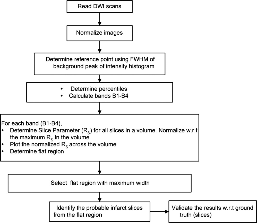
Algorithm

Get Radiology Tree app to read full this article<

Stage 1: Identification of infarct slices

Get Radiology Tree app to read full this article<

Concept of the algorithm

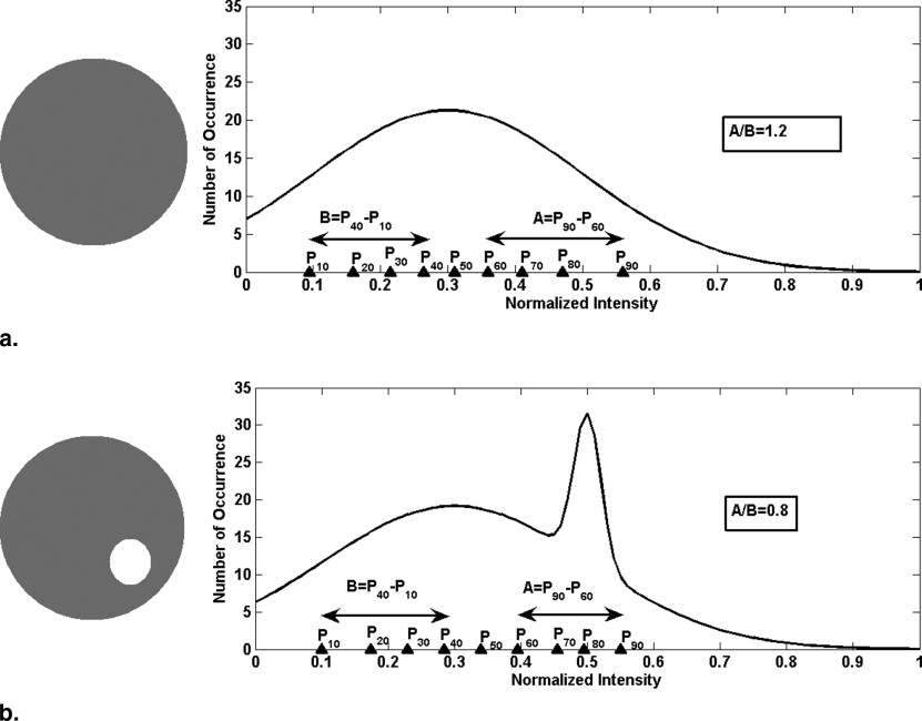
Get Radiology Tree app to read full this article<

Normalization of image

Get Radiology Tree app to read full this article<

Inorm=f*I−IminImax−Imin I

−

min

⁡

max

⁡

−

min

⁡

where I max and I min are the maximum and minimum intensity on a given slice and f is the normalization parameter. In our study, we selected f = 1 so that the maximum intensity is 1 and the minimum intensity is 0. The histograms of all the images have been plotted with 256 bins.

Get Radiology Tree app to read full this article<

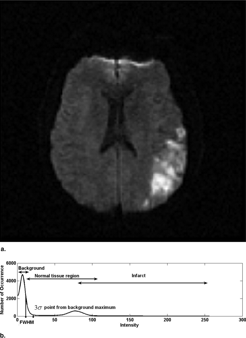
Reference point and slice parameter R s

Get Radiology Tree app to read full this article<

Rs=(1P50)(Pa+20−PaPb+20−Pb) R

(

)

(

−

)

where P a are percentiles in a slice above P 50 and P b are percentiles below P 50 .

Get Radiology Tree app to read full this article<

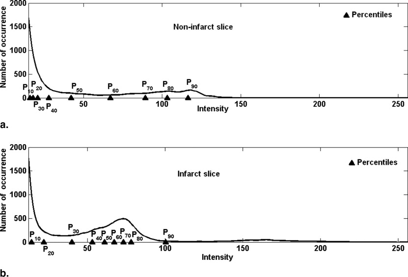
R s for different bands

Get Radiology Tree app to read full this article<

NormalizedRs=(Rs−min[Rs])/(max[Rs]−min[Rs]) Normalized

(

−

min

[

]

)

(

max

[

]

−

min

[

]

)

Get Radiology Tree app to read full this article<

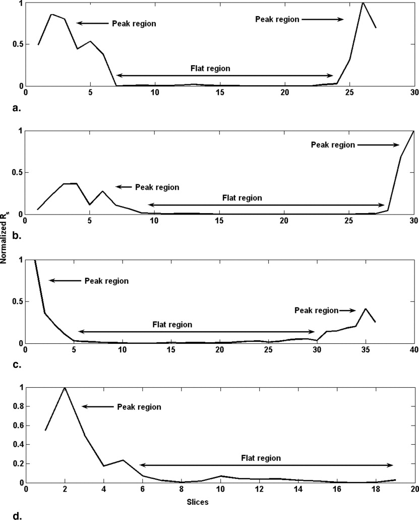
Occurrence of peaks and flat region

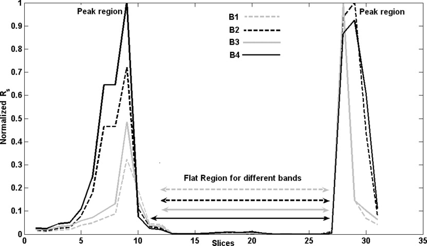
Get Radiology Tree app to read full this article<

Final width of flat region=[max (width of flat region in B1−B4)] Final width of flat region

[

max (width of flat region in B1

−

)

]

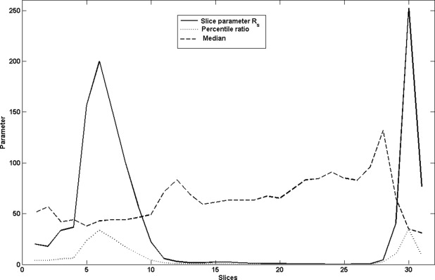
In the example discussed ( Fig 5 ), the extrema of flat region for B1 is at 12 and 28, for B2 at 12 and 28, for B3 at 12 and 28 and for B4 at 11 and 28. The maximum width corresponds to B4 (28 − 11 = 17), so we take the final extrema of flat region as 11 to 28.

Get Radiology Tree app to read full this article<

Hypothesis of flat region and infarct slices

Get Radiology Tree app to read full this article<

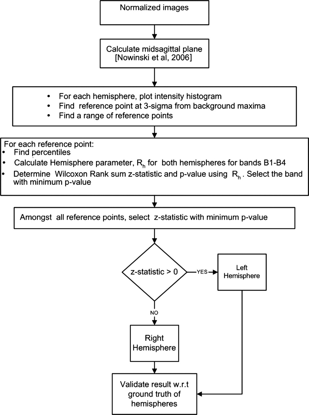
Stage 2: Localization of Infarct Hemisphere

Get Radiology Tree app to read full this article<

Selection of reference point (r i )

Get Radiology Tree app to read full this article<

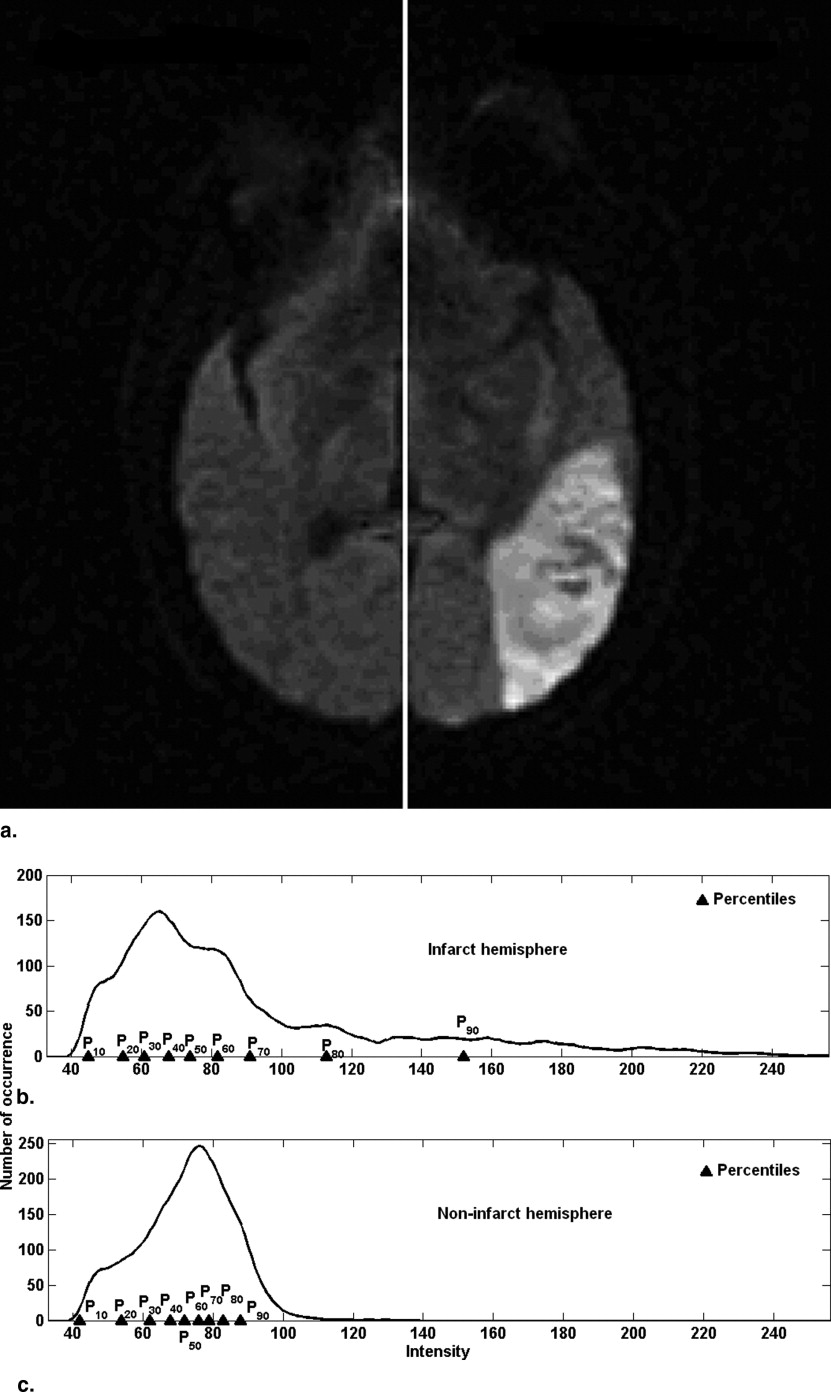
Percentile characteristics and hemisphere parameter R h

Get Radiology Tree app to read full this article<

Rh=P50(Pa+20−PaPb+20−Pb) R

(

−

)

Also a higher value of P 50 is observed in case of the infarct hemisphere. Multiplying by P 50 enhances the difference of Hemisphere parameter between the infarct (noninfarct) hemispheres.

Get Radiology Tree app to read full this article<

R h for infarct and noninfarct hemisphere

Get Radiology Tree app to read full this article<

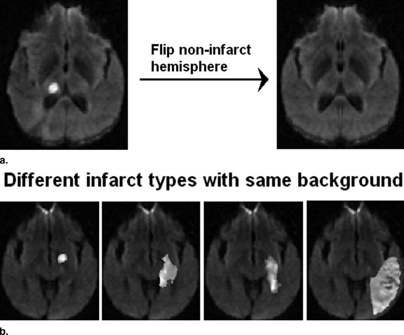
Synthetic Data Creation for Accuracy Estimation

Slice identification

Get Radiology Tree app to read full this article<

Hemisphere identification

Get Radiology Tree app to read full this article<

Results

Slice Identification

Get Radiology Tree app to read full this article<

Hemisphere Identification

Get Radiology Tree app to read full this article<

Table 1

Results of Hemisphere Identification

Case GT AR 1 L L 2 R R 3 L R 4 R R 5 R R 6 R R 7 L L 8 L L 9 R R 10 L L 11 L L 12 L L 13 L L 14 R R 15 R R 16 R R 17 R R 18 R R 19 R R 20 L L 21 R R 22 R R 23 L L 24 L L 25 R R 26 R R 27 R R 28 L L 29 L R 30 R R 31 L L 32 L L 33 R L 34 R R 35 L L 36 L L

GT: ground truth, AR: Algorithm result, L: Left hemisphere, R: Right Hemisphere.

Get Radiology Tree app to read full this article<

Accuracy of the Algorithm

Slice identification

Get Radiology Tree app to read full this article<

Hemisphere identification

Get Radiology Tree app to read full this article<

Discussion

Get Radiology Tree app to read full this article<

Infarct Slice Detection

Get Radiology Tree app to read full this article<

Infarct Hemisphere Detection

Get Radiology Tree app to read full this article<

Limitations and Further Improvements

Get Radiology Tree app to read full this article<

Potential

Get Radiology Tree app to read full this article<

Conclusion

Get Radiology Tree app to read full this article<

Appendix

Testing for Peak Location

Get Radiology Tree app to read full this article<

Location of Flat Region

Get Radiology Tree app to read full this article<

if slope>−0.01, extrema=x_i else consider [x_i+1:x_i+3] if slope

−

0.01

, extrema

x_i else consider [x_i+1:x_i+3]

Get Radiology Tree app to read full this article<

References

1. Menezes N.M., Ay H., Wang Zhu M., et. al.: The real estate factor: quantifying the impact of infarct location on stroke severity. Stroke 2007; 38: pp. 194-197.
2. Martel A.L., Allder S.J., Delay G.S., et. al.: Measurement of infarct volume in infarct patients using adaptive segmentation of diffusion weighted MR images. MICCAI 1999; 1679: pp. 22-31.
3. Li W., Li E., et. al.: Robust unsupervised segmentation of infarct lesion from diffusion tensor MR images using multiscale statistical classification and partial volume voxel reclassification. Neuroimage 2004; 23: pp. 1507-1518. J Tan
4. Bhanu Prakash K.N., Gupta V., Bilello M., et. al.: Identification, segmentation and image property study of acute infarcts in diffusion-weighted images by using a probabilistic neural network and adaptive gaussian mixture model. Acad Radiol 2006; 13: pp. 1474-1484.
5. Bhanu Prakash KN, Gupta V, Nowinski WL. Segmenting infarct in diffusion weighted imaging volumes. PCT/SG2006/000292, filed 3 October 2006.
6. Nowinski W.L., Bhanu Prakash K.N., Volkau I., et. al.: Rapid and automatic calculation of the midsagittal plane in magnetic resonance diffusion and perfusion images. Acad Radiol 2006; 13: pp. 652-663.
7. Nowinski W.L., Qian G., Bhanu Prakash K.N., et. al.: A CAD system for stroke MR and CT.2006.pp. 789. 92 Radiological Society of North America Scientific Assembly and Annual Meeting Program 2006, Chicago, IL: 25 November–1 December
8. Bezdec J.C.: Pattern recognition with fuzzy objective function algorithms.1981.Plenum PressNew York
9. Weisstein EW. Gaussian function. Available online from MathWorld: http://mathworld.wolfram.com/GaussianFunction.html
10. Gibbons J.D.: Nonparametric statistical inference.ed 21985.M. Dekker
11. Mann H.B., Whitney D.R.: On a test of whether one of 2 random variables is stochastically larger than the other. Annals of Mathematical Statistics 1947; 18: pp. 50-60.
12. Linn S.: A new conceptual approach to teaching the interpretation of clinical tests. J Stat Educ 2004; 12: Available online from: www.amstat.org/publications/jse/v12n3/linn.html
13. Zou K.H., Warfield S.K., Bharatha A., et. al.: Statistical validation of image segmentation quality based on spatial overlap index. Acad Radiol 2004; 11: pp. 178-189.
14. Kinnard L.M., Lo S.C.B., Duckett E., et. al.: Mass segmentation of dense breasts on digitized mammograms: Analysis of probability-based function. Medical Imaging 2005; 5747: pp. 1813-1823. Image Processing. Proceedings of the SPIE 2005
15. Hanley J.A., McNeil B.J.: The meaning and use of area under a receiver operating characteristic (ROC) curve. Radiology 1982; 143: pp. 29-36.
16. Moritani T., Ekholm S., Westesson P.L.: Diffusion weighted MR imaging of the brain.2005.Springer-VerlagBerlin
17. Bammer R., Markl M., Barnett A., et. al.: Analysis and generalized correction of the effect of spatial gradient field distortions in diffusion-weighted imaging. Magnet Reson Med 2003; 20: pp. 560-569.
18. Nowinski W.L., Qian G., Bhanu Prakash K.N., et. al.: Analysis of ischemic stroke MR images by means of brain atlases of anatomy and blood supply territories. Acad Radiol 2006; 13: pp. 1025-1034.
19. Nowinski W.L., Thirunavuukarasuu A.: The Cerefy clinical brain atlas on CD-ROM.2004.ThiemeNew York

Automatic and Rapid Identification of Infarct Slices and Hemisphere in DWI Scans

Rationale and Objectives

Materials and Methods

Results

Conclusions

Materials and methods

Data Acquisition

Data Description

Algorithm

Stage 1: Identification of infarct slices

Concept of the algorithm

Normalization of image

Reference point and slice parameter R s

R s for different bands

Occurrence of peaks and flat region

Hypothesis of flat region and infarct slices

Stage 2: Localization of Infarct Hemisphere

Selection of reference point (r i )

Percentile characteristics and hemisphere parameter R h

R h for infarct and noninfarct hemisphere

Synthetic Data Creation for Accuracy Estimation

Slice identification

Hemisphere identification

Results

Slice Identification

Hemisphere Identification

Accuracy of the Algorithm

Slice identification

Hemisphere identification

Discussion

Infarct Slice Detection

Infarct Hemisphere Detection

Limitations and Further Improvements

Potential

Conclusion

Appendix

Testing for Peak Location

Location of Flat Region

References

Further Reading

Abstracts of Funded National Institutes of Health Grants (January)

Analysis of Heart Rate and Heart Rate Variation During Cardiac CT Examinations

Automatic Prediction of Infarct Growth in Acute Ischemic Stroke from MR Apparent Diffusion Coefficient Maps