Automatic Identification of the Reference System Based on the Fourth Ventricular Landmarks in T1-weighted MR Images

Rationale and Objectives

The reference system based on the fourth ventricular landmarks (including the fastigial point and ventricular floor plane) is used in medical image analysis of the brain stem. The objective of this study was to develop a rapid, robust, and accurate method for the automatic identification of this reference system on T1-weighted magnetic resonance images.

Materials and Methods

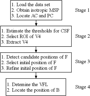
The fully automated method developed in this study consisted of four stages: preprocessing of the data set, expectation-maximization algorithm–based extraction of the fourth ventricle in the region of interest, a coarse-to-fine strategy for identifying the fastigial point, and localization of the base point. The method was evaluated on 27 Brain Web data sets qualitatively and 18 Internet Brain Segmentation Repository data sets and 30 clinical scans quantitatively.

Results

The results of qualitative evaluation indicated that the method was robust to rotation, landmark variation, noise, and inhomogeneity. The results of quantitative evaluation indicated that the method was able to identify the reference system with an accuracy of 0.7 ± 0.2 mm for the fastigial point and 1.1 ± 0.3 mm for the base point. It took <6 seconds for the method to identify the related landmarks on a personal computer with an Intel Core 2 6300 processor and 2 GB of random-access memory.

Conclusion

The proposed method for the automatic identification of the reference system based on the fourth ventricular landmarks was shown to be rapid, robust, and accurate. The method has potentially utility in image registration and computer-aided surgery.

With the further development of image guidance, the frequency of stereotactic interventions in the brain stem is increasing . The issue of localization in the brain stem is now, more than ever, a topic of importance, as modern neuroscience collects huge amounts of data that often have no meaning without precise descriptions of location. In addition, many structures in the brain stem are invisible in neuroimages, and the method of indirect (or atlas-based) localization is often used by functional neurosurgeons referring to a certain reference system. Therefore, a reference system is a prerequisite for accurate localization in the brain stem.

The most widely used reference system is based on the anterior commissure (AC) and the posterior commissure (PC) (the AC-PC reference system), which is referred to by two well-known stereotactic human brain atlases . The primary concern of these two atlases is to aid neuroradiologists and neurosurgeons in locating specific structures in the core brain, not the brain stem but the basal ganglia, that lie close to the AC and PC. Another alternative reference system is based on the fourth ventricular landmarks B and F (the B-F reference system), which is referred to by Afshar et al’s brain stem atlas. This atlas describes a variability study of the brain stem structures. The landmark F is the fastigial point of the fourth ventricle (V4). The landmark Ba is the intersection point of the line tangential to the fourth ventricular floor (VFL) and the line passing F and orthogonal to the VFL. Figure 1 illustrates the definition of two reference systems on the midsagittal plane (MSP). Theoretically, greater proximity of the origin of the reference system to the structure has a positive impact on the precise determination of their spatial relation. A local coordinate system is particularly useful for assigning exact locations to distribution data . Zrinzo et al reported that the anteroposterior coordinate of the caudal pole of pedunculopontine nucleus (PPN) has significantly greater variance in relation to the AC-PC reference system than to the B-F reference system ( F test, P < .001), while the variances of the superoinferior and lateral coordinates have no significant difference. Therefore, the B-F reference system can be used for location in the brain stem.

Open full size image

Figure 1

Definition of the B-F reference system (dashed line) and AC-PC reference system (solid line) on the MSP. The vertical dashed line is the VFL, and the horizontal dashed line passes the fastigial point F and intersects with the VFL at the base point B. AC, anterior commissure; MSP, midsagittal plane; PC, posterior commissure; VFL, ventricular floor.

Get Radiology Tree app to read full this article<

Materials and methods

Data Overview

Get Radiology Tree app to read full this article<

Method

Get Radiology Tree app to read full this article<

Stage 1: Preprocessing of the Data Set

Get Radiology Tree app to read full this article<

Stage 2: Segmentation of V4

Get Radiology Tree app to read full this article<

P(X|uk,σk)=12π√σk×exp{−(X−uk)22σ2k}, P

(

)

exp

{

−

(

−

)

}

where k denotes the tissue type, u k is the mean, and σ k is the standard deviation. Then the histogram f ( X ) can be approximated by a sum of equation 1 :

f(X)=∑5k=1Zk∫P(X|uk,vk)dX, f

(

)

∑

∫

(

)

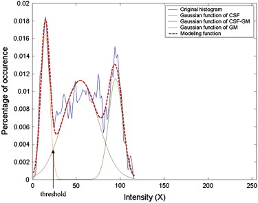
where Z k is the proportional coefficient. The expectation-maximization algorithm then seeks the solution of maximizing the expectation. In this study, the number of tissues in the ROI is limited and known, which can be used as a priori knowledge. Because there is little WM in the ROI, which can be ignored, the number of tissue types is truncated to three: CSF, CSF-GM, and GM. The k -means algorithm is used to estimate initial means of each class. Figure 4 shows the results of multiple Gaussian functions fitting to the original histogram using the expectation-maximization algorithm.

Get Radiology Tree app to read full this article<

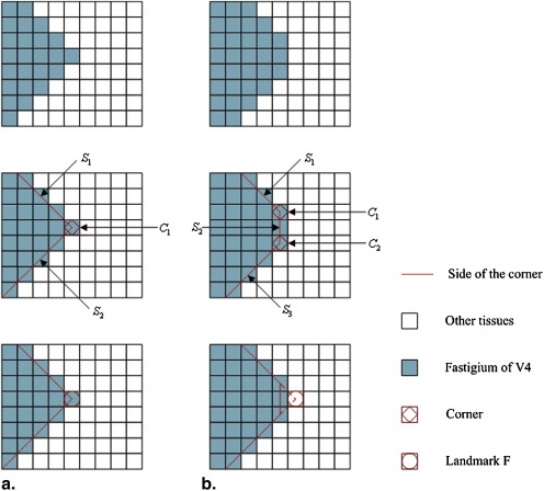
Stage 3: Identification of the Landmark F

Get Radiology Tree app to read full this article<

Stage 4: Identification of the Landmark B

Get Radiology Tree app to read full this article<

Results

Get Radiology Tree app to read full this article<

Table 1

Location Error for Landmarks B and F in CS-30 and IBSR-18

B F Data Set Maximum (mm) Average (mm) Maximum (mm) Average (mm) CS-30 2.0 0.9 1.4 0.6 IBSR-18 2.5 1.3 1.7 0.8

B, base point; CS-30, 30 clinical T1-weighted magnetic resonance brain volumes; F, fastigial point; IBSR-18, 18 high-resolution real volumes from the Internet Brain Segmentation Repository.

Table 2

Location Error for Landmarks B and F in BW-27

B F Parameter Maximum (mm) Average (mm) Maximum (mm) Average (mm) Slice thickness (mm) 1 1.5 0.6 1.0 0.5 3 2.5 1.7 2.1 1.1 5 4.1 2.3 2.5 1.5 RF 20% 1.8 0.7 1.5 0.6 40% 2.4 1.0 2.0 0.8 Noise 5% 1.6 0.8 1.5 0.6 9% 2.7 0.9 2.5 0.8

B, base point; BW-27, 27 Brain Web phantom data sets; F, fastigial point; RF, intensity nonuniformity.

Get Radiology Tree app to read full this article<

Table 3

Location Error for Landmarks B and F on the MSP of one IBSR-18 Data Set for Different Positions of AC and PC

Statistic B F Maximum (mm) 0.9 0.5 Average (mm) 0.9 0.5

AC, anterior commissure; B, base point; F, fastigial point; IBSR-18, 18 high-resolution real volumes from the Internet Brain Segmentation Repository; MSP, midsagittal point; PC, posterior commissure.

Get Radiology Tree app to read full this article<

Table 4

Statistics of the Location Error of Two Experts for the Landmarks B and F in All Data Sets of CS-30

Expert 1 Expert 2 Expert 1 + Expert 2 Landmark Maximum (mm) Average (mm) Maximum (mm) Average (mm) Maximum (mm) Average (mm) B 3.5 1.9 2.8 1.7 1.9 1.1 F 2.1 0.8 1.9 0.7 1.5 0.5

B, base point; CS-30, 30 clinical T1-weighted magnetic resonance brain volumes; F, fastigial point.

Get Radiology Tree app to read full this article<

Discussion

Get Radiology Tree app to read full this article<

References

1. Kondziolka D., Lunsford L.D.: Results and expectations with image-integrated brainstem stereotactic biopsy. Surg Neurol 1995; 43: pp. 558-562.
2. Zrinzo L., Zrinzo L.V., Tisch S., et. al.: Stereotactic localization of the human pedunculotontine nucleus: atlas-based coordinates and validation of a magnetic resonance imaging protocol for direction localization. Brain 2008; 131: pp. 1588-1598.
3. Talairach J., Tournoux P.: Coplanar stereotactic atlas of the human brain.1988.Thieme MedicalNew York
4. Schaltenbrand G., Hassler R.G., Wahren W.: Atlas for stereotaxy of the human brain.1977.Thieme MedicalStuttgart, Germany
5. Afshar F., Watkins E.S., Yap J.C.: Stereotaxic atlas of the human brainstem and cerebellar nuclei: A variability study.1978.RavenNew York
6. Bjaalie J.G.: Localization in the brain: new solutions emerging. Nat Rev Neurosci 2002; 3: pp. 322-325.
7. Rohr K.: On 3D differential operators for detecting point landmarks. Image Vision Comput 1997; 15: pp. 219-233.
8. Förstner W.: A feature based correspondence algorithm for image matching. Intern Arch Photogram Remote Sens 1986; 26: pp. 150-166.
9. Liu J., Gao W., Huang S., Nowinski W.L.: A model-based, semi-global segmentation approach for automatic 3-D point landmark localization in neuroimages. IEEE Trans Med Imaging 2008; 27: pp. 1034-1044.
10. Hu Q., Nowinski W.L.: A rapid algorithm for robust and automatic extraction of the midsagittal plane of the human cerebrum from neuroimages based on local symmetry and outlier removal. Neuroimage 2003; 20: pp. 2153-2165.
11. Prakash K.N.B., Hu Q., Aziz A., Nowinski W.L.: Rapid and automatic localization of the anterior and posterior commissure point landmarks in MR volumetric neuroimages. Acad Radiol 2006; 13: pp. 36-54.
12. Demster A.P., Laird N.M., Rubin D.B.: Maximum likelihood from incomplete data via the EM algorithm. J R Stat Soc 1977; 39: pp. 1-38.
13. Smith S.M., Brady J.M.: SUSAN—a new approach to low level image processing. Int J Comput Vision 1997; 23: pp. 45-78.
14. Chaudhuri D., Samal A.: A simple method for fitting of bounding rectangle to closed regions. Patt Recogn 2007; 40: pp. 1981-1989.
15. Fu Y., Gao W., Zhu M., et. al.: Computer-assisted automatic localization of the human pendunculopontine nucleus in T1-weighted MR images: A Preliminary study. Int J Med Robotics Comput Assist Surg 2009; In Press

Automatic Identification of the Reference System Based on the Fourth Ventricular Landmarks in T1-weighted MR Images

Rationale and Objectives

Materials and Methods

Results

Conclusion

Materials and methods

Data Overview

Method

Stage 1: Preprocessing of the Data Set

Stage 2: Segmentation of V4

Stage 3: Identification of the Landmark F

Stage 4: Identification of the Landmark B

Results

Discussion

References

Further Reading

Cerebral Cavernous Hemangiomas at 7 Tesla

Comparison of 2D and 3D Views for Evaluation of Flat Lesions in CT Colonography

Detecting Epidermal Growth Factor Receptor Tumor Activity In Vivo During Cetuximab Therapy of Murine Gliomas