Automatic Model-guided Segmentation of the Human Brain Ventricular System From CT Images

Rationale and Objectives

Accurate segmentation of the brain ventricular system on computed tomographic (CT) imaging is useful in neurodiagnosis and neurosurgery. Manual segmentation is time consuming, usually not reproducible, and subjective. Because of image noise, low contrast between soft tissues, large interslice distance, large shape, and size variations of the ventricular system, no automatic method is presently available. The authors propose a model-guided method for the automated segmentation of the ventricular system.

Materials and Methods

Fifty CT scans of patients with strokes at different sites were collected for this study. Given a brain CT image, its ventricular system was segmented in five steps: (1) a predefined volumetric model was registered (or deformed) onto the image; (2) according to the deformed model, eight regions of interest were automatically specified; (3) the intensity threshold of cerebrospinal fluid was calculated in a region of interest and used to segment all regions of cerebrospinal fluid from the entire brain volume; (4) each ventricle was segmented in its specified region of interest; and (5) intraventricular calcification regions were identified to refine the ventricular segmentation.

Results

Compared to ground truths provided by experts, the segmentation results of this method achieved an average overlap ratio of 85% for the entire ventricular system. On a desktop personal computer with a dual-core central processing unit running at 2.13 GHz, about 10 seconds were required to analyze each data set.

Conclusion

Experiments with clinical CT images showed that the proposed method can generate acceptable results in the presence of image noise, large shape, and size variations of the ventricular system, and therefore it is potentially useful for the quantitative interpretation of CT images in neurodiagnosis and neurosurgery.

Because of its relatively short scanning time and low cost, computed tomographic (CT) imaging is widely used in neurosurgery and neurodiagnosis . To better analyze brain CT scans, segmentation of the ventricular system may be of importance for several reasons. First, the ventricular system is useful for the diagnosis of human brain abnormality: ventricular enlargement can be associated with some diseases, such as schizophrenia, ventriculitis, and meningitis. Second, information about the position, shape, and size of the ventricular system is helpful for locating ventricular hemorrhages and staging and treatment evaluation of brain stroke . Because the intensity of the ischemic region on a CT scan is usually between the cerebrospinal fluid (CSF) and gray matter (GM), and can even be overlapped with CSF regions, the accurate segmentation of the ventricular system is useful for ischemic region localization. Third, the segmented ventricular system can be used as an important anatomic landmark to guide the registration of a brain atlas such as the Talairach and Tournoux (TT) atlas with CT scans and thus to increase registration accuracy.

A number of methods have been developed for the extraction of the ventricular system from magnetic resonance images, for example, intensity-based methods such as thresholding and region growing , model-based methods such as atlas warping , geometric and parametric model deformation , and knowledge-based methods . However, no method is presently available for the automatic segmentation of the ventricular system from CT scans. This is due mainly to the following difficulties.

Get Radiology Tree app to read full this article<

Open full size image

Figure 1

Histogram enhancement for cerebrospinal fluid (CSF) segmentation: (a) histogram of the whole computed tomographic scan; (b) histogram of whole brain tissue inside the brain skull: it is not suitable to segment the CSF in the brain, because the CSF peak is not distinguishable; and (c) local histogram calculated in the vicinity of the ventricular system: its CSF peak is enhanced and visible and is used to find the threshold of the CSF using Gaussian function fitting. GM, gray matter; WM, white matter.

Get Radiology Tree app to read full this article<

Open full size image

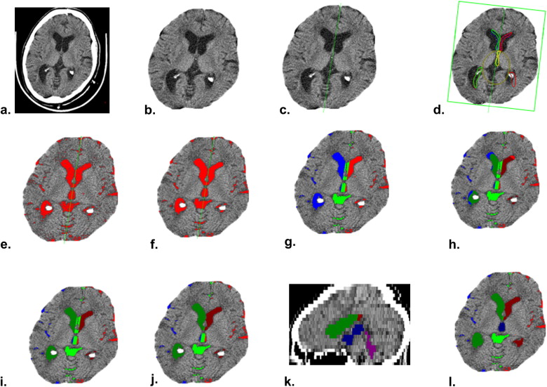
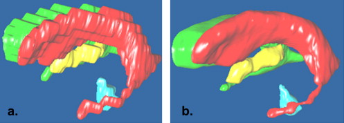
Figure 2

Illustration of original images and segmentation results of subjects with different morphometric and pathologic features. The first row shows the original images of four subjects. The second row shows their segmentation results. The third row displays the three-dimensional models built from the segmentation results of the entire ventricles. (a) Subject with a large ischemic region adjacent to right ventricle. (b) Subject with very small ventricles. (c) Subject with serious intraventricular calcification. (d) Subject with very large ventricles.

Get Radiology Tree app to read full this article<

Open full size image

Figure 3

Illustration of ventricular leakage problems: the third ventricle has a wide common boundary (region A1) with the lateral ventricle and leaks to the subarachnoid cavity at its posterior-inferior part (region A2); the lateral ventricle (region A3) leaks to the basal cistern through the region (A4) on its inferior neighboring slice.

Get Radiology Tree app to read full this article<

Materials and Methods

Get Radiology Tree app to read full this article<

Construction of the ROI Model

Get Radiology Tree app to read full this article<

Registration of ROI Model to Image

Get Radiology Tree app to read full this article<

Generation of ROI in Image

Get Radiology Tree app to read full this article<

Ω0=V0∪Ω(V′5,−d1), Ω

∪

(

′

−

)

Ωi=Ω(V′i,d2)−Ω0fori=1,2;Ωi=Ω(V′i,d2)fori=3,4, Ω

(

′

)

−

for

;

(

′

)

for

Ω5=V10−Ω0;Ω6=V20−Ω0, Ω

−

;

−

and

Ω7=Ω(V′1∪V′2,d2), Ω

(

′

∪

′

)

where d 1 and d 2 are given constants with their values empirically set to 4 and 6 mm, respectively. Region Ω 0 is used to avoid the leakage of the two lateral ventricles, region Ω 7 is used to calculate the CSF intensity threshold, and regions Ω 1 to Ω 6 are used for the segmentation of four ventricles.

Get Radiology Tree app to read full this article<

Calculation of the CSF Threshold

Get Radiology Tree app to read full this article<

f(x)=∑2i=1hiexp[(x−μi)2/(2σ21)], f

(

)

∑

exp

[

(

−

)

(

)

]

where x is the intensity value, μ the mean, σ the standard deviation, and h the height of the Gaussian function.

Get Radiology Tree app to read full this article<

Segmentation of the Ventricular System

Get Radiology Tree app to read full this article<

Identification of Intraventricular Calcification

Get Radiology Tree app to read full this article<

Results

Get Radiology Tree app to read full this article<

Table 1

Comparison Between Our Ventricular Segmentation Results and Ground Truth on Images With Different Representative Features

Left Ventricle Right Ventricle Third Ventricle Fourth Ventricle Four Ventricles Subject DSC FP FN DSC FP FN DSC FP FN DSC FP FN DSC FP FN 1 82.1 0.3 30.1 70.4 36.5 15.0 60.1 23.2 47.0 74.2 23.3 27.2 74.1 21.6 22.5 2 87.2 4.6 19.1 84.4 2.0 25.6 47.0 83.9 12.8 57.7 82.7 5.6 78.3 14.1 20.2 3 78.6 0.5 35.0 85.6 14.3 14.4 74.4 29.8 23.1 70.6 41.3 23.0 82.2 10.1 23.2 4 96.1 2.2 7.4 96.4 0.8 6.9 92.0 13.1 8.6 96.4 6.5 6.9 96.3 1.3 7.1 5 92.1 0.4 14.3 90.1 0.2 17.8 51.7 32.1 54.4 46.3 20.8 63.6 90.1 1.1 17.1 6 83.7 3.2 25.7 80.2 0.8 32.5 80.2 17.7 21.2 73.1 19.1 31.4 80.9 5.4 28.5 7 92.5 0.8 13.2 92.2 1.1 13.5 78.9 35.7 11.7 80.7 5.9 28.4 91.5 2.7 13.4 8 82.1 31.5 8.4 78.7 37.6 4.2 66.2 72.2 14.7 31.3 79.3 48.1 78.9 36.8 7.6 9 75.7 32.0 13.6 74.2 41.3 10.8 49.6 89.5 31.1 51.8 76.6 3.3 72.1 40.1 13.1 10 81.2 8.9 25.6 81.5 7.3 26.2 74.9 19.2 28.6 88.7 1.8 18.9 81.0 9.0 25.9 11 81.2 8.6 25.8 79.1 7.8 29.5 69.9 22.6 34.2 79.9 34.1 10.9 79.4 10.7 27.1 12 86.8 6.9 18.0 86.3 7.3 18.6 75.2 49.1 10.2 83.8 11.5 19.6 85.8 9.3 17.9 13 63.9 19.1 44.1 77.3 23.6 22.1 63.7 85.7 13.2 77.2 37.5 13.7 71.1 27.1 29.8 14 89.0 4.2 16.4 90.2 2.5 15.8 76.1 9.3 32.9 66.0 10.6 45.5 88.5 3.8 17.5

DSC, Dice similarity coefficient; FP, false-positive ratio; FN, false-negative ratio.

Table 2

Performance Statistics of Our Method on the Entire Data Set ( n = 50)

Left Ventricle Right Ventricle Third Ventricle Fourth Ventricle Four Venticles DSC FP FN DSC FP FN DSC FP FN DSC FP FN DSC FP FN Mean 85.0 6.1 16.2 85.8 8.37 17.2 67.5 41.8 27.8 58.8 42.9 38.6 84.8 10.1 18.0 Standard deviation 7.8 9.5 10.3 6.8 15.5 7.8 18.3 38.1 19.9 29.7 49.6 31.5 7.1 12.8 7.5

DSC, Dice similarity coefficient; FP, false-positive ratio; FN, false-negative ratio.

Get Radiology Tree app to read full this article<

Discussion

Statistical Versus Structural Method

Get Radiology Tree app to read full this article<

Shape-based Interpolation

Get Radiology Tree app to read full this article<

Limitations and Further Improvement

Get Radiology Tree app to read full this article<

Conclusion

Get Radiology Tree app to read full this article<

Appendix

boundary Patch–based Region-Growing Procedure

Get Radiology Tree app to read full this article<

∂i,k+1=∪p∈∂i,k{q|q∈N26(p),q∈Ω}−[K∪(∪ni=1∂i,k)](k=0,1,2,…), ∂

∪

∈

∂

{

∈

(

)

∈

}

−

[

∪

(

∪

∂

)

]

(

…

)

where N 26 ( p ) represents all the 26 neighbors of the voxel p . The procedure of generating ∂ i , k +1 from ∂ i , k continues either until ∂i,ki+1 ∂

1 is empty or the number of voxels in ∂i,ki+1 ∂

1 is more than twice the number of voxels in the previous step ∂i,ki ∂

i (ie, # ∂i,ki+1 ∂

1 > 2 × # ∂i,ki ∂

i ). The last stopping condition is used to avoid leakage.

Get Radiology Tree app to read full this article<

X=∪ni=1(∪kij=0∂i,j)∪K. X

∪

(

∪

∂

)

∪

The region X is regarded as the result of the region-growing procedure. For the ventricular segmentation, the candidate region Ω is the related CSF region.

Get Radiology Tree app to read full this article<

References

1. Hu X., Jiang X., Zhou X., et. al.: Risks of intracranial hemorrhage in patients with Parkinson’s disease receiving deep brain stimulation and ablation. Parkinsonism Relat Disord 2010; 16: pp. 96-100.
2. Liu F., Qian J., Lu Y.: Computer-assisted stereotactic neurosurgery with framework neurosurgery navigation. Clin Neurol Neurosurg 2008; 110: pp. 696-700.
3. Nowinski W.L., Qian G., Prakash K.N.B., et. al.: Stroke Suite: CAD systems for acute ischemic stroke, hemorrhagic stroke, and stroke in ER. Med Imaging Informatics 2008; 4987: pp. 377-386.
4. Talairach J., Tournoux P.: Coplanar stereotactic atlas of the human brain.1988.ThiemeStuttgart, Germany
5. Worth A.J., Makris N., Patti M.R., et. al.: Precise segmentation of the lateral ventricles and caudate nucleus in MR brain images using anatomically driven histograms. IEEE Trans Med Imaging 1998; 17: pp. 303-310.
6. Schnack H.G., Hulshoff P.H.E., Baare W.F.C., Viergever M.A., Kahn R.S.: Automatic segmentation of the ventricular system from MR images of the human brain. Neuroimage 2001; 14: pp. 95-104.
7. Sonka M., Tadikonda S.K., Collins S.M.: Knowledge-based interpretation of MR brain images. IEEE Trans Med Imaging 1996; 15: pp. 443-452.
8. Xia Y., Hu Q., Aziz A., Nowinski W.L.: A knowledge-driven algorithm for a rapid and automatic extraction of the human cerebral ventricular system for MR meuroimages. Neuroimage 2004; 21: pp. 269-282.
9. Holden M., Schnable J.A., Hill D.L.G.: Quantifying small changes in brain ventricular volume using non-rigid registration. Lecture Notes Comput Sci 2010; 2208: pp. 49-56.
10. Baillard C., Hellier P., Barillot C.: Segmentation of 3D brain structures using level sets and dense registration. IEEE Workshop Math Methods Biomed Image Anal 2000; pp. 94-101.
11. Kaus M.R., Warfield S.K., Nabavi A., Black P.M., Jolesz F.A., Kikinis R.: Automated segmentation of MR images of brain tumors. Radiology 2001; 218: pp. 586-591.
12. Shen D., Herskovits E.H., Davatzikos C.: An adaptive-focus statistical shape model for segmentation and shape modeling of 3-D brain structure. IEEE Trans Med Imaging 2001; 20: pp. 257-270.
13. Liu J., Huang S., Nowinski W.L.: Automatic segmentation of the human brain ventricles in MR images by knowledge-based region growing and trimming. Neuroinformatics 2009; 7: pp. 131-146.
14. Han X., Fischl B.: Atlas renormalization for improved brain MR image segmentation across scanner platforms. IEEE Trans Med Imaging 2007; 26: pp. 479-486.
15. Showalter C., Clymer B.D., Richmond B., Powell K.: Three-dimensional texture analysis of cancellous bone cores evaluated at clinical CT resolutions. Osteoporosis Int 2006; 17: pp. 259-266.
16. Al-Kadi O.S., Watson D.: Texture analysis of aggressive and nonaggressive lung tumor CE CT images. IEEE Trans Biomed Eng 2008; 55: pp. 1822-1830.
17. Liu J., Nowinski W.L.: A hybrid approach to shape-based interpolation of stereotactic atlases of the human brain. Neuroinformatics 2006; 4: pp. 177-198.
18. Liu J., Gao W., Huang S., Nowinski W.L.: A model-based, semi-global segmentation approach for automatic 3D point landmark localization in neuroimages. IEEE Trans Med Imag 2008; 27: pp. 1034-1044.
19. Mangin J.F., Frouin V., Bloch I., Regis J., Lopez-Krahe J.: From 3D magnetic resonance images to structural representations of the cortex topography using topology preserving deformations. J Math Imag Vision 1995; 5: pp. 297-318.
20. Volkau I., Bhanu Prakash K.N., Anand A., Aziz A., Nowinski W.L.: Extraction of the midsagittal plane from morphological neuroimages using the Kullback-Leibler’s measure. Med Image Anal 2006; 10: pp. 863-874.
21. Maurer C.R., Qi J.R., Raghavan V.: A linear time algorithm for computing exact Euclidean distance transforms of binary images in arbitrary dimensions. IEEE Trans PAMI 2003; 25: pp. 265-270.
22. Gonzalez R.C., Woods R.E.: Digital Image Processing.1993.Addison-WesleyBoston
23. Liu J., Huang S., Aziz A., Nowinski W.L.: Three dimensional digital atlas of the orbit constructed from multi-modal radiological images. Int J Comput Assist Radiol Surg 2007; 1: pp. 275-283.
24. Liu J., Huang S., Nowinski W.L.: A hybrid approach for segmentation of anatomic structures in medical images. Int J Comput Assist Radiol Surg 2008; 3: pp. 213-219.
25. Nowinski W.L., Qian G., Prakash K.N.B., Hu Q., Aziz A.: Fast Talairach transformation for magnetic resonance neuroimages. J Comput Assist Tomogr 2006; 30: pp. 629-641.

Automatic Model-guided Segmentation of the Human Brain Ventricular System From CT Images

Rationale and Objectives

Materials and Methods

Results

Conclusion

Materials and Methods

Construction of the ROI Model

Registration of ROI Model to Image

Generation of ROI in Image

Calculation of the CSF Threshold

Segmentation of the Ventricular System

Identification of Intraventricular Calcification

Results

Discussion

Statistical Versus Structural Method

Shape-based Interpolation

Limitations and Further Improvement

Conclusion

Appendix

boundary Patch–based Region-Growing Procedure

References

Further Reading

Academic Memories

An Approach to Comparing Accuracies of Two Flair MR Sequences in the Detection of Multiple Sclerosis Lesions in the Brain in the Absence of Gold Standard

Cardiac Imaging Training in Radiology Residency Programs