
Rationale and Objectives
Although segmentation algorithms for cerebrospinal fluid (CSF), white matter (WM), and gray matter (GM) on unenhanced computed tomographic (CT) images exist, there is no complete research in this area. To take into account poor image contrast and intensity variability on CT scans, the aim of this study was to derive and validate a novel, automatic, adaptive, and robust algorithm.
Materials and Methods
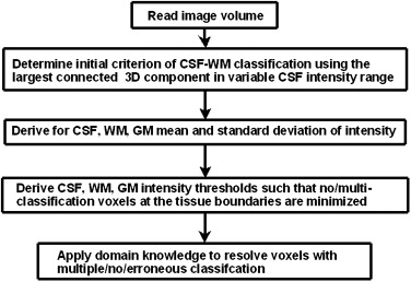
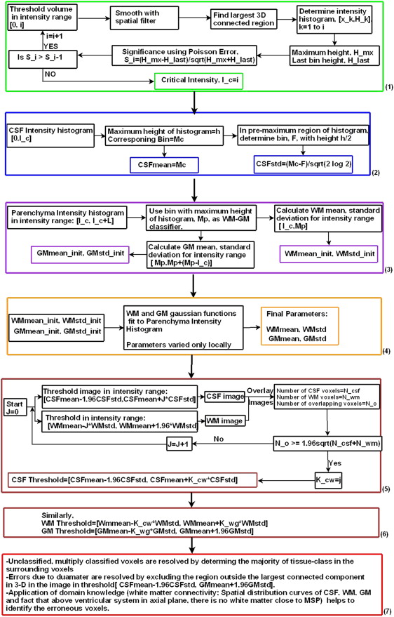
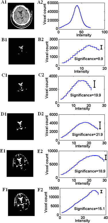
Unenhanced CT scans of normal subjects from two different centers were used. The algorithm developed uses adaptive thresholding, connectivity, and domain knowledge and is based on heuristics on the shape of CT histogram. The slope of the intensity histogram corresponding to the three-dimensional largest connected region in a variable CSF intensity range is tracked to determine the critical intensity, which serves as an initial classifier of CSF-WM. Thresholds of CSF, WM, and GM are then optimally derived to minimize classification overlap. Multiple, null, and erroneous classifications are resolved by applying domain knowledge.
Results
The ground-truth regions with the minimal partial volume effect were used to evaluate segmentation results using the statistical markers. Average sensitivity, Dice index, and specificity, respectively, for the first center were 95.7%, 97.0%, and 98.6% for CSF; 96.1%, 97.3%, and 98.8% for WM; and 95.2%, 94.3%, and 92.8% for GM. The results were consistent for the second data center.
Conclusions
The algorithm automatically identifies CSF, WM, and GM on unenhanced CT images with high accuracy, is robust to data from different scanners, does not require any parameter setting, and takes about 5 minutes in MATLAB to process a 512 × 512 × 30 scan. The algorithm has potential use in research and clinical applications.
Although segmentation algorithms for unenhanced computed tomographic (CT) images of the brain exist, there is still a need for an accurate and robust solution. Some of the associated reasons are low contrast between different tissues (cerebrospinal fluid [CSF], white matter [WM], and gray matter [GM]), diffuse tissue boundaries, artifacts due to the partial volume, inhomogeneity in images, and lack of validation due to difficulty in achieving the accurate ground truth (GT), among others . Intensity variations may further occur because of different scanner parameters combined with signal attenuations (due to different skull thickness) or beam hardening artifacts. Therefore, hard-coded threshold values for CT imaging of different tissues can lead to substantial errors in CT segmentation. Furthermore, pathologic conditions may also be responsible for the loss of GM and WM contrast on CT images (eg, in comatose patients after cardiac arrest ).
In the literature, only a few methods for CSF, WM, and GM segmentation of CT scans have been reported. The method of Lee et al is based on k -means and expectation maximization clustering, which basically clusters the intensities into k clusters. The intensity belongs to the cluster with the nearest mean. The performance of clustering algorithms, however, is sensitive to the choice of initial parameters . Also, the focus of Lee et al’s study was only on CSF, skull, parenchyma, and calcification, not on the segmentation of WM and GM. Another approach by Hu and Xie is an automatic segmentation method based on a combination of pattern recognition, fuzzy theory, anatomy, fractal dimensions, and parameter thresholds. Although this algorithm was validated on 10 CT images (986 slices), there was no quantitative measure of the performance. The algorithm classifies CSF, WM, and GM but does not handle their diffuse boundaries. In general, a shape-based or texture-based analysis can perform well only when image quality is good. A genetic algorithm to locate the boundary of an organ in medical images was proposed by Heydarian et al . However, their method has limitations when an organ is composed of different tissue types (eg, the brain). Although genetic algorithms are a possible solution to medical image segmentation, there can be issues with parameter initialization, convergence criteria, and computation time . Segmentation methods based only on intensity thresholds, such as that of DeLeo et al , can have limitations due to the partial volume effect. Another fully automatic algorithm, by Ruttimann et al , focuses only on the segmentation of CSF regions.
Get Radiology Tree app to read full this article<
Get Radiology Tree app to read full this article<
Materials and methods
Get Radiology Tree app to read full this article<
Get Radiology Tree app to read full this article<
Get Radiology Tree app to read full this article<
Get Radiology Tree app to read full this article<
Get Radiology Tree app to read full this article<
Get Radiology Tree app to read full this article<
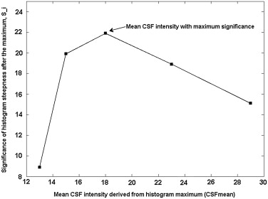
Estimation of the Initial Criterion of CSF-WM Classification: Critical Intensity
Get Radiology Tree app to read full this article<
Get Radiology Tree app to read full this article<
Get Radiology Tree app to read full this article<
Get Radiology Tree app to read full this article<
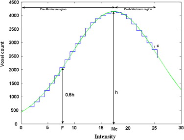
Estimation of CSF Parameters
Get Radiology Tree app to read full this article<
Get Radiology Tree app to read full this article<
Get Radiology Tree app to read full this article<
Get Radiology Tree app to read full this article<
WM and GM parameters
Get Radiology Tree app to read full this article<
Get Radiology Tree app to read full this article<
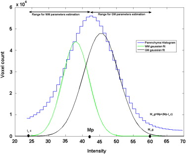
Get Radiology Tree app to read full this article<
Get Radiology Tree app to read full this article<
Intensity Thresholds
Get Radiology Tree app to read full this article<
Get Radiology Tree app to read full this article<
Get Radiology Tree app to read full this article<
Get Radiology Tree app to read full this article<
Get Radiology Tree app to read full this article<
Get Radiology Tree app to read full this article<
Spatial errors
Get Radiology Tree app to read full this article<
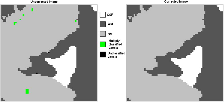
Get Radiology Tree app to read full this article<
Get Radiology Tree app to read full this article<
Get Radiology Tree app to read full this article<
Domain knowledge
Get Radiology Tree app to read full this article<
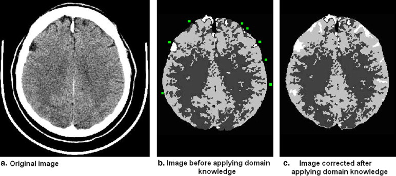
Get Radiology Tree app to read full this article<
Get Radiology Tree app to read full this article<
Results
Overlap of GT Regions with Segmented Volume
Get Radiology Tree app to read full this article<
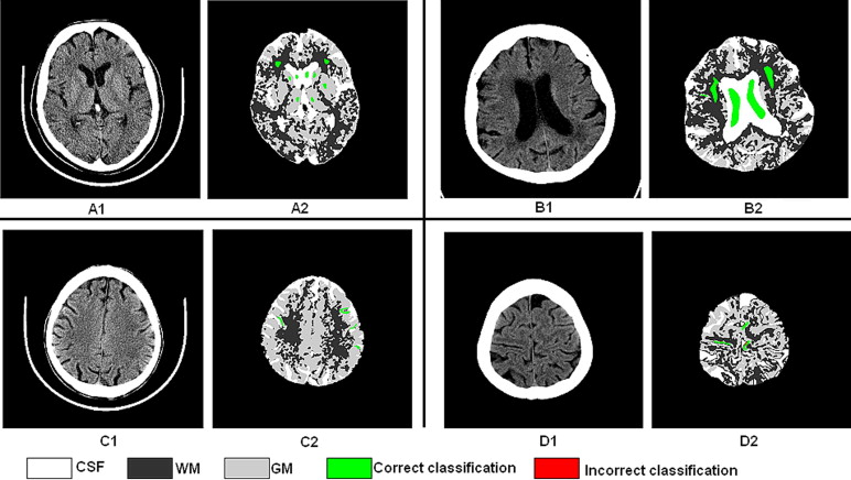
Table 1
Sensitivity, Dice Index , and Specificity of Ground Truth Comparison
Class Sensitivity (%) Dice Index (%) Specificity (%) Data from Poznań (70 data sets) CSF 95.7 97.0 98.6 WM 96.1 97.3 98.8 GM 95.2 94.3 92.8 Data from Kraków (14 data sets) CSF 95.2 96.1 98.5 WM 96.1 97.2 98.3 GM 95.9 94.7 93.3
CSF, cerebrospinal fluid; GM, gray matter; WM, white matter.
Get Radiology Tree app to read full this article<
Comparison of Mean Intensity of CSF, WM, and GM
Get Radiology Tree app to read full this article<
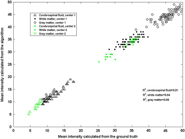
Get Radiology Tree app to read full this article<
Discussion
Get Radiology Tree app to read full this article<
Get Radiology Tree app to read full this article<
Get Radiology Tree app to read full this article<
Get Radiology Tree app to read full this article<
Get Radiology Tree app to read full this article<
Get Radiology Tree app to read full this article<
Get Radiology Tree app to read full this article<
Conclusions
Get Radiology Tree app to read full this article<
Acknowledgment
Get Radiology Tree app to read full this article<
Get Radiology Tree app to read full this article<
References
1. Pham D.L., Xu C., Prince J.L.: Current methods in medical image segmentation. Annu Rev Biomed Eng 2000; 2: pp. 315-337.
2. Torbey M.T., Selim M., Knorr J., et. al.: Quantitative analysis of the loss of distinction between gray and white matter in comatose patients after cardiac arrest. Stroke 2000; 31: pp. 2163-2167.
3. Lee T.H., Fauzi M.F.A., Komiya R.: Segmentation of CT brain images using K-means and EM clustering. Proc Comput Graph Imaging Visualiz Modern Techn Appl 2008; pp. 339-344.
4. Davenport J.W., Bezdek J.C., Hathaway R.J.: Parameters estimation for finite mixture distributions. Comput Math Appl 1988; 15: pp. 810-828.
5. Hu Y., Xie M.: Automatic segmentation of brain CT image based on multiplicate features and decision tree. Proc Int Conf Commun Circuit Syst 2007; pp. 837-840.
6. Heydarian M., Noseworthy M.D., Kamath M.V., et. al.: Optimizing the level set algorithm for detecting object edges in MR and CT images. IEEE Trans Nucl Sci 2009; 56: pp. 156-166.
7. Maulik U.: Medical image segmentation using genetic algorithms. IEEE Trans Inform Technol Biomed 2009; 13: pp. 166-173.
8. DeLeo J.M., Schwarz M., Creasy H., et. al.: Computer assisted categorization of brain computerized tomography pixels into cerebrospinal fluid, white matter and gray matter. Comput Biomed Res 1985; 18: pp. 79-88.
9. Ruttimann U.E., Joyce E.M., Rio D.E., et. al.: Fully automated segmentation of cerebrospinal fluid in computed tomography. Psychiatry Res Neuroimaging 1993; 50: pp. 101-119.
10. Klauschen F., Goldman A., Barra V., et. al.: Evaluation of automated brain MR image segmentation and volumetry methods. Hum Brain Mapping 2009; 30: pp. 1310-1327.
11. Hacker H., Artmann H.: The calculation of CSF spaces in CT. Neuroradiology 1978; 16: pp. 190-192.
12. Zimmerman R.A., Gibby W.A., Raymond F.: Neuroimaging: Clinical and Physical Principles.1999.SpringerNew York
13. Mandel J.: The Statistical Analysis of Experimental Data.1984.Courier Dover PublicationsNew York
14. Bevington P.R.: Data Reduction and Error Analysis for the Physical Sciences.1969.McGraw-HillNew York
15. Zou K.H., Warfield S.K., Bharatha A., et. al.: Statistical validation of image segmentation quality based on spatial overlap index. Acad Radiol 2004; 11: pp. 178-189.
16. Nowinski W.L., Qian G., Bhanu Prakash K.N., et. al.: Stroke suite: CAD systems for acute ischemic stroke, hemorrhagic stroke, and stroke in ER. Med Imaging Informat Lect Notes Comput Sci 2008; 4987: pp. 377-386.