Breast Mass Segmentation in Mammography Using Plane Fitting and Dynamic Programming

Rationale and Objectives

Segmentation is an important and challenging task in a computer-aided diagnosis (CAD) system. Accurate segmentation could improve the accuracy in lesion detection and characterization. The objective of this study is to develop and test a new segmentation method that aims at improving the performance level of breast mass segmentation in mammography, which could be used to provide accurate features for classification.

Materials and Methods

This automated segmentation method consists of two main steps and combines the edge gradient, the pixel intensity, as well as the shape characteristics of the lesions to achieve good segmentation results. First, a plane fitting method was applied to a background-trend corrected region-of-interest (ROI) of a mass to obtain the edge candidate points. Second, dynamic programming technique was used to find the “optimal” contour of the mass from the edge candidate points. Area-based similarity measures based on the radiologist’s manually marked annotation and the segmented region were employed as criteria to evaluate the performance level of the segmentation method. With the evaluation criteria, the new method was compared with 1) the dynamic programming method developed by Timp and Karssemeijer, and 2) the normalized cut segmentation method, based on 337 ROIs extracted from a publicly available image database.

Results

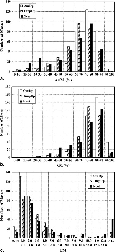
The experimental results indicate that our segmentation method can achieve a higher performance level than the other two methods, and the improvements in segmentation performance level were statistically significant. For instance, the mean overlap percentage for the new algorithm was 0.71, whereas those for Timp’s dynamic programming method and the normalized cut segmentation method were 0.63 ( P < .001) and 0.61 ( P < .001), respectively.

Conclusions

We developed a new segmentation method by use of plane fitting and dynamic programming, which achieved a relatively high performance level. The new segmentation method would be useful for improving the accuracy of computerized detection and classification of breast cancer in mammography.

Breast cancer is one of the leading causes of death in women . Scientific evidence indicates that early detection and treatment of breast cancer can reduce the mortality and morbidity of patients . Mammography is widely considered as one of the most cost-effective methods to detect early breast cancer . Computer-aided diagnosis (CAD) systems can be useful in breast cancer screening programs with mammography by providing radiologists with a “second opinion.”

Segmentation of masses in mammography is an important and challenging task in a CAD system. Accurate segmentation could provide accurate lesion features and thus improve accuracy in lesion detection and characterization . Segmentation of masses overlapping with dense breast tissue is particularly difficult because mass boundaries may become obscured, irregular, and low in contrast. In recent years, many studies have been focused on segmentation of mass lesions in digital mammography. Petrick et al developed a segmentation method based on density-weighted contrast enhancement (DWCE), which incorporated adaptive filtering and edge detection. Zheng et al proposed a method for the detection of masses with an adaptive multi-layer topographic region growth algorithm. Comer et al used Markov random fields to segment masses in a mammogram based on texture information. Catarious et al applied an iterative routine based on gray level to do mass segmentation. Yuan et al proposed a dual-stage method for lesion segmentation on digital mammograms, which combined a radial gradient index (RGI) based segmentation method and an improved active contour model.

Get Radiology Tree app to read full this article<

Materials and methods

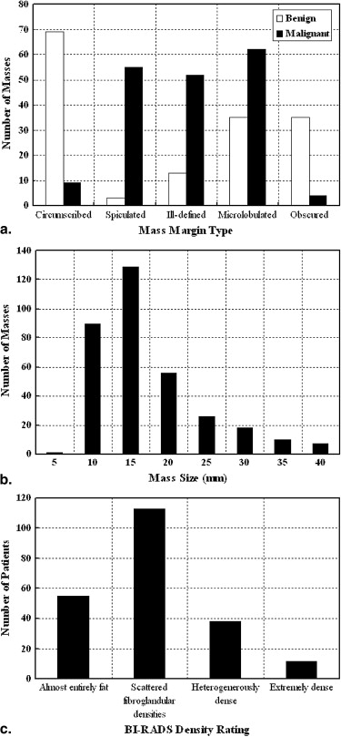
Dataset

Get Radiology Tree app to read full this article<

Segmentation Using Plane Fitting and Dynamic Programming

Get Radiology Tree app to read full this article<

Step 1: ROI Preprocessing

Get Radiology Tree app to read full this article<

Step 2: Detection of Edge Candidate Points by Use of Plane Fitting

Get Radiology Tree app to read full this article<

f=a⋅i+b⋅j+c, f

⋅

where −2≤i≤2 −

≤

2 and −2≤j≤2 −

≤

2 . Each pixel could thus be characterized by a set of three parameters “a,” “b,” and “c.” Because

⎧⎩⎨∂f∂i=a∂f∂j=b, {

∂

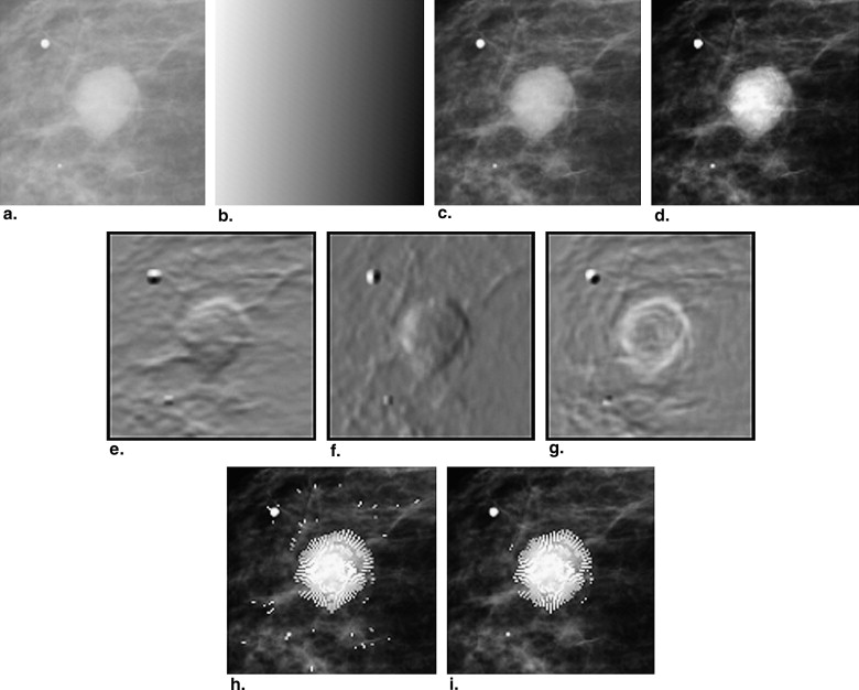
parameters “a” and “b” indicate the gradients on the vertical direction and the horizontal direction, respectively. Figure 3 e and f show the grayscale image corresponding to the vertical gradient and the horizontal gradient, respectively.

Get Radiology Tree app to read full this article<

{i=−tsinj=tcos. {

−

sin

cos

Get Radiology Tree app to read full this article<

f=−a⋅t⋅sin+b⋅t⋅cos+c, f

−

⋅

sin

⋅

cos

and consequently,

∂f∂t=−asin+bcos. ∂

∂

−

sin

cos

Get Radiology Tree app to read full this article<

Step 3: Delineation of Lesion Outline by Use of Dynamic Programming

Get Radiology Tree app to read full this article<

C(n)=dis(n,n−1)255−I(n), C

(

)

(

−

)

255

−

(

)

where dis( n , n – 1) represented the distance between the edge candidate point on the nth radial line and one edge candidate point on the (n – 1)th radial line, and I ( n ) represented the gray value of the edge candidate point on the nth radial line.

Get Radiology Tree app to read full this article<

Segmentation Using Dynamic Programming Proposed by Timp

Get Radiology Tree app to read full this article<

Segmentation Using Normalized Cut

Get Radiology Tree app to read full this article<

Segmentation Performance Evaluation

Get Radiology Tree app to read full this article<

AOM=Arearadiologist∩AreasegmentationArearadiologist∪Areasegmentation. A

log

∩

log

∪

Get Radiology Tree app to read full this article<

CM=(AOM+(1−Arearadiologist−Arearadiologist∩AreasegmentationArearadiologist)+(1−Areasegmentation−Arearadiologist∩AreasegmentationAreasegmentation))/3. C

(

−

log

−

log

∩

log

)

(

−

log

∩

)

Get Radiology Tree app to read full this article<

EM=Num(Arearadiologist∪Areasegmentation−Arearadiologist∩Areasegmentation)Num(perimeterradiologist), E

(

log

∪

−

log

∩

)

(

log

)

where Num(Arearadiologist∪Areasegmentation−Arearadiologist∩Areasegmentation) N

(

log

∪

−

log

∩

) represented the number of pixels in the mismatched area between the outline delineated by radiologists and the segmentation result, and Num ( perimeter radiologist ) represented the number of pixels on the outline delineated by the radiologists. The EM measures the accuracy of the segmentation algorithm relative to the actual size of the lesion. Unlike AOM and CM, the smaller the EM, the better the segmentation algorithm.

Get Radiology Tree app to read full this article<

Results

Get Radiology Tree app to read full this article<

Table 1

Descriptive Statistics of Performance Measures AOM, CM, and EM for the Three Segmentation Methods

Descriptive Statistics of AOM Method Min. First Qu. Median Mean Third Qu. Max. OurDp 0.098 0.665 0.736 0.712 0.803 0.921 TimpDp 0.003 0.547 0.651 0.627 0.747 0.902 Ncut 0.029 0.484 0.675 0.607 0.769 0.907

Descriptive Statistics of CM Method Min. First Qu. Median Mean Third Qu. Max. OurDp 0.399 0.766 0.816 0.801 0.867 0.946 TimpDp 0.080 0.691 0.764 0.743 0.829 0.934 Ncut 0.093 0.635 0.775 0.722 0.843 0.937

Descriptive Statistics of EM Method Min. First Qu. Median Mean Third Qu. Max. OurDp 0.614 1.487 2.093 2.762 3.154 22.191 TimpDp 0.733 1.719 2.796 3.962 4.416 43.323 Ncut 0.617 1.801 2.870 5.691 6.080 54.462

AOM, area overlap measure; CM, combined metric; EM, error metric.

Get Radiology Tree app to read full this article<

Table 2

P Values of the Two-sided Wilcoxon (rank-sum) Test for the Statistical Differences in the Three Area-based Similarity Measures (AOM, CM, and EM) of the Three Segmentation Methods

Method_P_ Value for AOM_P_ Value for CM_P_ Value for EM OurDp - TimpDp <.001 <.001 <.001 OurDp - Ncut <.001 <.001 <.001 TimpDp - Ncut 0.227 0.400 0.697

AOM, area overlap measure; CM, combined metric; EM, error metric; Ncut, normalised cut method; Our Dp, our method; Timp Dp, Timp’s method.

Get Radiology Tree app to read full this article<

Table 3

The Percentages of Masses with an Area Overlap Method of 0.6 or Higher for Five Subtlety Ratings (1: very subtle, 5: very obvious), and Five Mass Margin Types

Subtlety Rating Method 1 2 3 4 5 OurDp 80% 90% 85% 89% 86% TimpDp 60% 35% 66% 67% 70% Ncut 40% 50% 57% 58% 68%

Margin Type Method Circumscribed Spiculated Ill-defined Microlobulated Obscured OurDp 88% 78% 92% 84% 95% TimpDp 81% 48% 78% 59% 64% Ncut 56% 52% 75% 63% 64%

Ncut, normalised cut method; Our Dp, our method; Timp Dp, Timp’s method.

Get Radiology Tree app to read full this article<

Discussion

Get Radiology Tree app to read full this article<

Conclusion

Get Radiology Tree app to read full this article<

Acknowledgment

Get Radiology Tree app to read full this article<

References

1. Jemal A.J., Siegel R., Ward E., et. al.: Cancer statistics, 2007. CA Cancer J Clin 2007; 57: pp. 43-66.
2. Feig S.A., D’Orsi C.J., Hendrick R.E., et. al.: American College of Radiology guidelines for breast cancer screening. AJR Am J Roentgenol 1998; 171: pp. 29-33.
3. Cady B., Michaelson J.S.: The life-sparing potential of mammographic screening. Cancer 2001; 91: pp. 1699-1703.
4. Bird R.E., Wallace T.W., Yankaskas B.C.: Analysis of cancers missed at screening mammography. Radiology 1992; 184: pp. 613-617.
5. Doi K., MacMahon H., Katsuragawa S.: Computer-aided diagnosis in radiology: potential and pitfalls. Eur J Radiol 1999; l31: pp. 97-109.
6. Huo Z., Giger M.L., Vyborny C.J., et. al.: Computerized classification of benign and malignant masses on digitized mammograms: a study of robustness. Acad Radiol 2000; 7: pp. 1077-1084.
7. Sahiner B., Chan H.P., Petrick N., et. al.: Improvement of mammographic mass characterization using spiculation measures and morphological features. Med Phys 2001; 28: pp. 1455-1465.
8. Cheng H.D., Shi X.J., Min R., et. al.: Approaches for automated detection and classification of masses in mammograms. Pattern Recognition 2006; 39: pp. 646-668.
9. Sahiner B., Petrick N., Chan H.P., et. al.: Computer-aided characterization of mammographic masses: accuracy of mass segmentation and its effects on characterization. IEEE Trans Med Imaging 2001; 20: pp. 1275-1284.
10. Petrick N., Chan H.P., Wei D., et. al.: Automated detection of breast masses on mammograms using adaptive contrast enhancement and texture classification. Med Phys 1996; 23: pp. 1685-1696.
11. Zheng B., Chang Y.H., Gur D.: Computer detection of masses in digitized mammograms using single-image segmentation and a multilayer topographic feature analysis. Acad Radiol 1995; 2: pp. 959-966.
12. Comer M.L., Liu S., Delp E.J.: Statistical segmentation of mammograms. Presented at: Digital Mammography.Doi K.International Congress Series.1996.ElsevierAmsterdam, The Netherlands:pp. 471-474.
13. Catarious D.M., Baydush A.H., Floyd C.E.: Incorporation of an iterative, linear segmentation routine into a mammographic mass CAD system. Med Phys 2004; 31: pp. 1512-1520.
14. Yuan Y., Giger M.L., Li H., et. al.: A dual-stage method for lesion segmentation on digital mammograms. Med Phys 2007; 34: pp. 4180-4193.
15. Amini A.A., Weymouth T.E., Jain R.C.: Using dynamic programming for solving variational problem in vision. IEEE Trans Pattern Anal Mach Intell 1990; 12: pp. 855-867.
16. Yamada H., Merritt C., Kasvand T.: Recognition of kidney glomerulus by dynamic programming matching method. IEEE Trans Pattern Anal Mach Intell 1988; 10: pp. 731-737.
17. Nuyts J., Suetens P., Oosterlinck A., et. al.: Delineation of ECT images using global constraints and dynamic programming. IEEE Trans Med Imaging 1991; 10: pp. 489-498.
18. Aoyama M., Li Q., Katsuragawa S., et. al.: Computerized scheme for determination of the likelihood measure of malignancy for pulmonary nodules on low-dose CT images. Med Phys 2003; 30: pp. 387-394.
19. Timp S., Karssemeijer N.: A new 2D segmentation method based on dynamic programming applied to computer aided detection in mammography. Med Phys 2004; 31: pp. 958-971.
20. Domínguez A.R., Nandi A.K.: Improved dynamic-programming-based algorithms for segmentation of masses in mammograms. Med Phys 2007; 34: pp. 4256-4269.
21. Wang J., Engelmann R., Li Q.: Segmentation of pulmonary nodules in three-dimensional CT images by use of a spiral-scanning technique. Med Phys 2007; 34: pp. 4678-4689.
22. Fracheboud J., deKoning H.J., Beemsterboer P.M.M., et. al.: Nation-wide breast cancer screening in The Netherlands: results of initial and subsequent screening 1990-1995. Int J Cancer 1998; 75: pp. 694-698.
23. Suckling J., Parker J., Dance D., et. al.: The Mammographic Image Analysis Society digital mammogram database. Presented at: Exerpta Medica. International Congress Series 1994; 1069: pp. 375-378. Available at: http://peipa.essex.ac.uk/info/mias.html
24. Heath M., Bowyer K.W., Kopans D., et. al.: Current status of the digital database for screening mammography.Karssemeijer N.Thijssen M.Hendriks J.Presented at: Digital Mammograpy.1998.Kluwer, DordrechtBoston, MA:pp. 457-460. Available at: http://marathon.csee.usf.edu/
25. Shi J., Malik J.: Normalized cuts and image segmentation. IEEE Trans Pattern Anal Mach Intell 2000; 22: pp. 888-905.
26. Heath M, Bowyer KW, Kopans D. The Digital Database for Screening Mammography. Presented at: 5th International Workshop on Digital Mammography. Toronto, Canada. June 2000.
27. American College of Radiology Breast Imaging Reporting and Data System Atlas (BI-RADS Atlas).4th ed.2003.American College of RadiologyReston, VA
28. Farid H.: Blind inverse γ correction. IEEE Trans Image Proc 2001; 10: pp. 1428-1433.
29. Image Segmentation with Normalized Cuts. Available at: http://www.cis.upenn.edu/∼jshi/software/ Accessed November 30, 2006
30. Kupinski M.A., Giger M.L.: Automated seeded lesion segmentation on digital mammograms. IEEE Trans Med Imaging 1998; 17: pp. 510-517.
31. Te Brake G.M., Karssemeijer N.: Segmentation of suspicious densities in digital mammograms. Med Phys 2001; 28: pp. 259-266.
32. Hammoude A.: An empirical parameter selection method for endocardial border identification algorithms. Comput Med Imaging Graph 2001; 25: pp. 33-45.

Breast Mass Segmentation in Mammography Using Plane Fitting and Dynamic Programming

Rationale and Objectives

Materials and Methods

Results

Conclusions

Materials and methods

Dataset

Segmentation Using Plane Fitting and Dynamic Programming

Step 1: ROI Preprocessing

Step 2: Detection of Edge Candidate Points by Use of Plane Fitting

Step 3: Delineation of Lesion Outline by Use of Dynamic Programming

Segmentation Using Dynamic Programming Proposed by Timp

Segmentation Using Normalized Cut

Segmentation Performance Evaluation

Results

Discussion

Conclusion

Acknowledgment

References

Further Reading

Atlas of Brain Function

Computed Radiography-based Mammography with 50-μm Pixel Size

Diffusion Tensor Tractography in the Head-and-Neck Reg ion Using a Clinical 3-T MR Scanner