
Rationale and Objectives
Based on the definitions in mass category of Breast Imaging Reporting and Data System developed by American College of Radiology, eight computerized features including shape, orientation, margin, lesion boundary, echo pattern, and posterior acoustic feature classes are proposed.
Materials and Methods
Our experimental database consists of 265 pathology-proven cases including 180 benign and 85 malignant masses. The capacity of each proposed feature in differentiating malignant from benign masses was validated by Student’s t test and the correlation between each proposed feature and the pathological result was evaluated by point biserial coefficient. Binary logistic regression model was used to relate all proposed features and pathological result as a computer-aided diagnosis (CAD) system. The diagnostic value of each proposed feature in the CAD system was further evaluated by the feature selection methods. Additionally, the likelihood of malignancy for each individual feature was also estimated by binary logistic regression.
Results
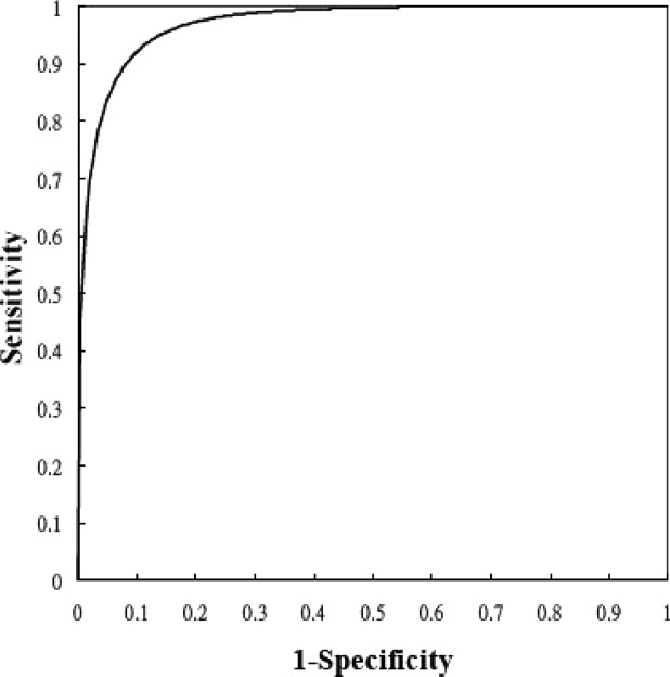
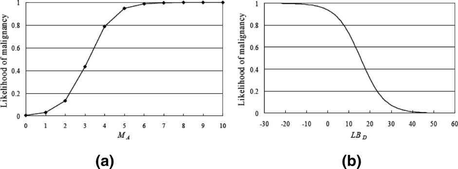
On each proposed feature, the malignant cases were significantly different from the benign ones. The correlation between the angular characteristic and pathological result was indicated as very high. Three substantial correlations appear in features irregular shape, undulation characteristic, and degree of abrupt interface, but the relationship for orientation feature is low. For the constructed CAD system, the performance indices accuracy, sensitivity, specificity, PPV, and NPV were 91.70% (243 of 265), 90.59% (77 of 85), 92.22% (166 of 180), 84.62% (77 of 91), and 95.40% (166 of 174), respectively, and the area index in the ROC analysis was 0.97. Compared with the significant contribution of angular characteristic, the diagnostic values of posterior acoustic feature and orientation feature were relatively low for the CAD system. When three or more angular characteristics are discovered or the degree of abrupt interface is lower than 18, the likelihood of malignancy could be predicted as greater than 40%.
Conclusion
The computerized BI-RADS sonographic features conform to the sign of malignancy in the clinical experience and efficiently help the CAD system to diagnose the mass.
Breast cancer is ranked as the second leading cause for cancer death in women after lung cancer by American Cancer Society ( ). The most useful way to reduce cancer deaths is early detection and treatment ( ). The introduction of mammography into medical usage helps physicians capture the visualized information in patients’ anatomy. Recently, ultrasound becomes an important alternative equipment for mammography in the evaluation of breast cancer because of its characteristics, including being noninvasive, more efficient, relatively inexpensive, real-time, and convenient ( ). Today, the developments of imaging techniques refine the quality of pictures and can greatly improve diagnostic accuracy for early detecting breast lesions so as to reduce the number of unnecessary biopsies ( ).
In the clinical diagnosis, feature detection plays a fundamental role in describing mass characteristics and could greatly affect the diagnostic result. Stavros et al. ( ) proposed several sonographic characteristics to describe a mass, such as ellipsoid shape, number of lobulations, ratio of wide to anteroposterior dimension, and posterior shadowing. With the rapid development of computer applications, most imaging tools rely on a computer-aided diagnosis (CAD) system to efficiently process the digitized data. Furthermore, a powerful function in differentiating malignant from benign lesions was developed and embedded into CAD system to assist the doctors in many researches ( ). Recently, Medipattern (Toronto, Canada) has also developed the first medical imaging software application, B-CAD, for analysis of the breast ultrasound images. In order to describe a mass in the computer system, the sonographic features are quantified into computerized sonographic features. For describing the formation of a mass, shape and margin characteristic classes could be adopted. The mass shape could be described by the moments and Fourier descriptors ( ) or several factors such as roundness, aspect-ratio, convexity, and solidity ( ). Madabhushi et al. ( ) and Kim et al. ( ) evaluated the shape irregularity by the direction of gradient magnitude and the derivative of curvature on each pixel of mass boundary, respectively. Joo et al. ( ) counted the spiculate characteristic of margin class by applying the Fourier transform on the polar coordinates constructed by the boundary pixels and the center of mass. Chen et al. ( ) counted the number of substantial protuberances and depressions on the margin by the convex hull. In addition to describing the mass formation, Drukker et al. ( ) detected the potential lesions based on expected mass shape and margin characteristics. Except for the formation of a mass, the correlation or dissimilarity between pixels of selected ROI or a mass are also useful to describe the mass characteristics. Texture analysis is a useful method to describe such features within selected ROI or a mass ( ). Kim et al. ( ) described acoustic differences within a mass by the distribution of gray scales. Furthermore, they evaluated the degree of definition of boundary by the gradient magnitudes. For estimating the clearness degree of mass boundary, Sehgal et al. ( ) partitioned the lesion boundary into N sectors and then comparing the difference significance between the inside and the outside of each sector. Horsch et al. ( ) partitioned the area behind a mass into three areas and the differences between these areas are used to measure the posterior acoustic feature.
Get Radiology Tree app to read full this article<
Get Radiology Tree app to read full this article<
Materials and methods
Data Acquisition
Get Radiology Tree app to read full this article<
Computerized BI-RADS Features
Get Radiology Tree app to read full this article<
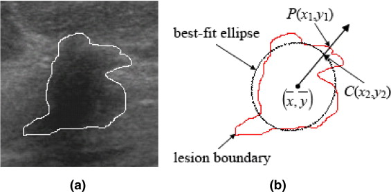
Shape Class
Get Radiology Tree app to read full this article<
D(P)=(x1−x2)2+(y1−y2)2−−−−−−−−−−−−−−−−−−√. D
(
P
)
=
(
x
1
−
x
2
)
2
+
(
y
1
−
y
2
)
2
.
Get Radiology Tree app to read full this article<
Get Radiology Tree app to read full this article<
SV=∑P∈LBD(P)LBN S
V
=
∑
P
∈
L
B
D
(
P
)
L
B
N
where P is any pixel on the lesion boundary and LB N denotes the number of pixels on the lesion boundary.
Get Radiology Tree app to read full this article<
Orientation Class
Get Radiology Tree app to read full this article<
OE=⎧⎩⎨⎪⎪⎪⎪⎪⎪⎪⎪⎪⎪π−−π2π−if0≤≤π2ifπ2<≤πifπ<≤3π2if3π2<≤2π. O
E
=
{
i
f
0
≤
≤
π
2
π
−
i
f
π
2
<
≤
π
−
π
i
f
π
<
≤
3
π
2
2
π
−
i
f
3
π
2
<
≤
2
π
.
Get Radiology Tree app to read full this article<
Margin Class
Get Radiology Tree app to read full this article<
N8(P)={(x−1,y−1),(x,y−1),(x+1,y−1),(x−1,y),(x+1,y),(x−1,y+1),(x,y+1),(x+1,y+1)} N
8
(
P
)
=
{
(
x
−
1
,
y
−
1
)
,
(
x
,
y
−
1
)
,
(
x
+
1
,
y
−
1
)
,
(
x
−
1
,
y
)
,
(
x
+
1
,
y
)
,
(
x
−
1
,
y
+
1
)
,
(
x
,
y
+
1
)
,
(
x
+
1
,
y
+
1
)
}
The distance from P to the lesion boundary is recursively defined as
Distance(P)=Min{Distance(N8(P))}+1 D
i
s
tan
c
e
(
P
)
=
M
i
n
{
D
i
s
tan
c
e
(
N
8
(
P
)
)
}
+
1
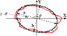
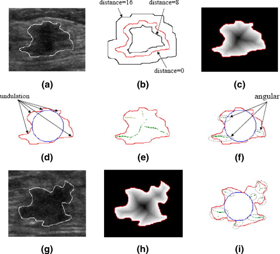
where Min { Distance ( N 8 ( P ))} denotes the minimum of known distance in P ’s eight neighbors. The distance for all boundary pixels are set to 0 as initial condition. An example for illustrating distance map is shown in Figure 3 b and 3 c. Then, a maximum inscribed circle inside the mass is found to extract the margin features from the distance map. By the maximum inscribed circle, some lobulate areas are clearly partitioned from the mass as shown in Figure 3 d. However, only the significant lobulate areas should be counted. Therefore, if the maximum distance within lobulate area is less than four, such area is regarded as slighter undulation and should be ignored. Then, the number of significant lobulate areas is defined as the undulation characteristics M U of margin class. Furthermore, the local maxima on the distance map could be used to detect the angular characteristics as shown in Figure 3 e. In order to count the number of angular characteristics M A , the local maxima in each lobulate area are grouped by their Euclidean coordinates as shown in Figure 3 f. In the grouping algorithm, the Euclidean distances from a new discovered local maximum to the center of each formed grouped local maxima are calculated. If the shortest distance is larger than a predefined threshold, the new discovered local maximum is regarded as a new grouped local maximum. Whereas, the new discovered local maximum is appended to the grouped local maxima which with the shortest distance and then the center of the modified grouped local maxima is recalculated. By experimentation, the predefined threshold is set to 10 in this study. In the grouping algorithm, those local maxima within the maximum inscribed circle would be ignored. For example, the local maxima located in the upper of mass were ignored as shown in Figure 3 e. Compared with the feature M U , the feature M A especially detects the angular characteristics on the margin as shown in Figure 3 i.
Get Radiology Tree app to read full this article<
Lesion Boundary Class
Get Radiology Tree app to read full this article<
avgTissue=∑kdistance(P)=1I(P)NTissueandavgMass=∑kdistance(P)=1I(P)NMass a
v
g
T
i
s
s
u
e
=
∑
d
i
s
tan
c
e
(
P
)
=
1
k
I
(
P
)
N
T
i
s
s
u
e
a
n
d
a
v
g
M
a
s
s
=
∑
d
i
s
tan
c
e
(
P
)
=
1
k
I
(
P
)
N
M
a
s
s
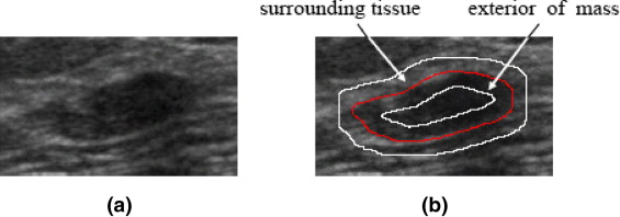
where I ( P ) is the gray intensity of pixel P , N Tissue denotes the number of pixels in the partitioned part of surrounding tissue, and N Mass represents the number of pixels in the outer mass. Then, the lesion boundary feature LB D for evaluating the degree of abrupt interface is defined as
LBD=avgTissue−avgMass. L
B
D
=
a
v
g
T
i
s
s
u
e
−
a
v
g
M
a
s
s
.
By experimentation, the width k is set to 3 in this study.
Get Radiology Tree app to read full this article<
Echo Pattern Class
Get Radiology Tree app to read full this article<
EPI=∑I(P)P∈MassNMass E
P
I
=
∑
I
(
P
)
P
∈
M
a
s
s
N
M
a
s
s
where I ( P ) is the gray intensity of mass pixel P and N Mass denotes the number of mass pixels.
Get Radiology Tree app to read full this article<
Get Radiology Tree app to read full this article<
GX(P)=I(x−1,y−1)+2*I(x−1,y)+I(x−1,y+1)−I(x+1,y−1)−2*I(x+1,y)−I(x+1,y+1) G
X
(
P
)
=
I
(
x
−
1
,
y
−
1
)
+
2
*
I
(
x
−
1
,
y
)
+
I
(
x
−
1
,
y
+
1
)
−
I
(
x
+
1
,
y
−
1
)
−
2
*
I
(
x
+
1
,
y
)
−
I
(
x
+
1
,
y
+
1
)
and
GY(P)=I(x−1,y−1)+2*I(x,y−1)+I(x+1,y−1)−I(x−1,y+1)−2*I(x,y+1)−I(x+1,y+1). G
Y
(
P
)
=
I
(
x
−
1
,
y
−
1
)
+
2
*
I
(
x
,
y
−
1
)
+
I
(
x
+
1
,
y
−
1
)
−
I
(
x
−
1
,
y
+
1
)
−
2
*
I
(
x
,
y
+
1
)
−
I
(
x
+
1
,
y
+
1
)
.
Then, the gradient magnitude on P is defined as
G(P)=GX(P)2+GY(P)2−−−−−−−−−−−−−−−√ G
(
P
)
=
G
X
(
P
)
2
+
G
Y
(
P
)
2
Finally, the internal echo pattern feature EP AG could be estimated by the average variation as
EPAG=∑G(P)P∈MassNMass. E
P
A
G
=
∑
G
(
P
)
P
∈
M
a
s
s
N
M
a
s
s
.
Get Radiology Tree app to read full this article<
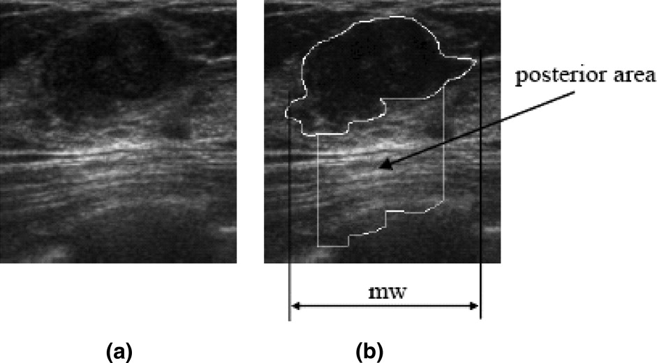
Posterior Acoustic Feature Class
Get Radiology Tree app to read full this article<
avgPA=∑I(P)P∈PANPA a
v
g
P
A
=
∑
I
(
P
)
P
∈
P
A
N
P
A
where I ( P ) is the gray intensity of pixel P in the posterior area and N PA denotes the number of pixels in the posterior area. Then, the posterior acoustic feature PS D is defined as
PSD=avgPA−EPI P
S
D
=
a
v
g
P
A
−
E
P
I
where EP I is defined in Equation 8.
Get Radiology Tree app to read full this article<
Experimental Method and Performance Evaluation
Get Radiology Tree app to read full this article<
Get Radiology Tree app to read full this article<
Accuracy=(TP+TN)/(TP+TN+FP+FN),Sensitivity=TP/(TP+TN),Specificity=TN/(TN+FP),PPV=TP/(TP+FP),andNPV=TN/(TN+FN). Accuracy
=
(
T
P
+
T
N
)
/
(
T
P
+
T
N
+
F
P
+
F
N
)
,
Sensitivity
=
TP
/
(
TP
+
T
N
)
,
Specificity
=
TN
/
(
T
N
+
F
P
)
,
PPV
=
TP
/
(
T
P
+
F
P
)
,
and
NPV
=
TN
/
(
T
N
+
F
N
)
.
where TP is the number of positives correctly classified as positive, TN is the number of negatives correctly classified as negative, FP is the number of negatives falsely classified as positive, and FN is the number of positives falsely classified as negative. Moreover, the ROC analysis is also used to evaluate the diagnostic performance. The ROCKIT software (C. Metz, University of Chicago, Chicago, IL) is used in the ROC analysis.
Get Radiology Tree app to read full this article<
Get Radiology Tree app to read full this article<
Get Radiology Tree app to read full this article<
Results
Data Analysis of Computerized BI-RADS Features
Get Radiology Tree app to read full this article<
Table 1
Mean Values and Standard Deviations (SDs) for the Benign and Malignant Groups
Class Feature Mean ± SD_P_ value_r pb_ Benign Malignant Shape_S V_ 16.75 ± 19.19 126.78 ± 130.49 <.001 0.56 Orientation_O E_ 11.93 ± 13.33 15.93 ± 17.75 <.05 0.12 Margin_M U_ 2.16 ± 0.87 3.52 ± 1.17 <.001 0.56M A 1.61 ± 1.01 4.56 ± 2.09 <.001 0.70 Lesion boundary_LB D_ 27.29 ± 10.45 13.18 ± 7.93 <.001 −0.57 Echo pattern_EP I_ 49.69 ± 13.82 39.09 ± 14.12 <.001 −0.35EP AG 48.30 ± 10.86 37.32 ± 8.59 <.001 −0.46 Posterior shadowing_PS D_ 42.02 ± 19.82 26.23 ± 27.12 <.001 −0.32
The significance for differentiating the benign from malignant group is verified by the Student’s t test. The strength of relationship between the pathological result and each proposed BI-RADS feature is evaluated by the point-biserial correlation coefficient r pb .
Get Radiology Tree app to read full this article<
Computer-Aided Diagnosis Using All Computerized BI-RADS Features
Get Radiology Tree app to read full this article<
Get Radiology Tree app to read full this article<
Get Radiology Tree app to read full this article<
Table 2
The Diagnostic Result of the CAD System
Pathology CAD system Total Benign Malignant Benign TN 166 FP 14 180 Malignant FN 8 TP 77 85 Total 174 91 265
Table 3
The Diagnostic Performance of the CAD System
Performance indices Rate Accuracy 91.70% Sensitivity 90.59% Specificity 92.22% PPV 84.62% NPV 95.40%
Get Radiology Tree app to read full this article<
Discussion
Diagnostic Value of Each Computerized BI-RADS Feature in the CAD System
Get Radiology Tree app to read full this article<
Table 4
The Diagnostic Value of Each Proposed Feature in the Diagnosis Function is Verified by the Feature Selection Methods
Step Forward selected Backward removed Feature_R_ 2 χ 2 Feature_R_ 2 χ 2 1M A 0.657 167.980 All 0.851 248.588 2LB D 0.731 27.870O E 0.851 −0.008 3EP I 0.779 19.675PS D 0.850 −0.533 4M U 0.805 11.474EP I 0.847 −1.747 5S V 0.845 18.709M U 0.830 −7.870 6EP AG 0.850 2.339S V 0.784 −20.641 7PS D 0.851 0.533EP AG 0.731 −21.939 8O E 0.851 0.008LB D 0.657 −27.870 9M A −167.980
When the feature is selected or removed at each step, the R 2 value indicates ability of CAD system for predicting the pathological result and the improvement compared to the previous step is evaluated by the χ 2 .
Get Radiology Tree app to read full this article<
Critical Thresholds on Angular and Degree of Abrupt Interface Characteristics
Get Radiology Tree app to read full this article<
Get Radiology Tree app to read full this article<
Get Radiology Tree app to read full this article<
Get Radiology Tree app to read full this article<
Conclusion and future works
Get Radiology Tree app to read full this article<
Get Radiology Tree app to read full this article<
References
1. Jemal A., Siegel R., Ward E., et. al.: Cancer statistics, 2006. CA Cancer J Clin 2006; 56: pp. 106-130.
2. American Cancer Society: 2006.American Cancer SocietyAtlanta, GA
3. American Cancer Society: 2006.American Cancer SocietyAtlanta, GA
4. Baker J.A., Soo M.S.: Breast US: Assessment of technical quality and image interpretation. Radiology 2002; 223: pp. 229-238.
5. Rizzatto G.J.: Towards a more sophisticated use of breast ultrasound. Eur Radiol 2001; 11: pp. 2425-2435.
6. Williams J.C.: US of solid breast nodules. Radiology 1996; 198: pp. 585.
7. Stavros A.t., Thickman D., Rapp C.L., et. al.: Solid breast nodules: Use of sonography to distinguish between benign and malignant lesions. Radiology 1995; 196: pp. 123-134.
8. Liang S., Rangayyan R.M., Desautels J.E.L.: Application of shape analysis to mammographic calcifications. IEEE Trans Med Imaging 1994; 13: pp. 263-274.
9. Chang R.F., Wu W.J., Moon W.K., et. al.: Automatic ultrasound segmentation and morphology based diagnosis of solid breast tumors. Breast Cancer Res Treat 2005; 89: pp. 179-185.
10. Madabhushi A., Metaxas D.N.: Combining low-, high-level and empirical domain knowledge for automated segmentation of ultrasonic breast lesions. IEEE Trans Med Imaging 2003; 22: pp. 155-169.
11. Kim K.G., Cho S.W., Min S.J., et. al.: Computerized scheme for assessing ultrasonographic features of breast masses. Acad Radiol 2005; 12: pp. 58-66.
12. Joo S., Yang Y.S., Moon W.K., et. al.: Computer-aided diagnosis of solid breast nodules: Use of an artificial neural network based on multiple sonographic features. IEEE Trans Med Imaging 2004; 23: pp. 1292-1300.
13. Chen C.M., Chou Y.H., Han K.C., et. al.: Breast lesions on sonograms: Computer-aided diagnosis with nearly setting-independent features and artificial neural networks. Radiology 2003; 226: pp. 504-514.
14. Drukker K., Giger M.L., Vyborny C.J., et. al.: Computerized detection and classification of cancer on breast ultrasound. Acad Radiol 2004; 11: pp. 526-535.
15. Chang R.F., Wu W.J., Moon W.K., et. al.: Support vector machines for diagnosis of breast tumors on US images. Acad Radiol 2003; 10: pp. 189-197.
16. Chen D.R., Chang R.F., Huang Y.L.: Computer-aided diagnosis applied to US of solid breast nodules by using neural networks. Radiology 1999; 213: pp. 407-412.
17. Chang R.F., Wu W.J., Moon W.K., et. al.: Improvement in breast tumor discrimination by support vector machines and speckle-emphasis texture analysis. Ultrasound Med Biol 2003; 29: pp. 679-686.
18. Chen D.R., Chang R.F., Huang Y.L., et. al.: Texture analysis of breast tumors on sonograms. Semin Ultrasound CT MR 2000; 21: pp. 308-316.
19. Bader W., Bohmer S., van L.P., et. al.: Does texture analysis improve breast ultrasound precision?. Ultrasound Obstet Gynecol 2000; 15: pp. 311-316.
20. Kim K.G., Kim J.H., Min B.G.: Classification of malignant and benign tumors using boundary characteristics in breast ultrasonograms. J Digit Imaging 2002; 15: pp. 224-227.
21. Sehgal C.M., Cary T.W., Kangas S.A., Weinstein S.P., Schultz S.M., Arger P.H., Conant E.F.: Computer-based margin analysis of breast sonography for differentiating malignant and benign masses. J Ultrasound Med 2004; 23: pp. 1201-1209.
22. Horsch K., Giger M.L., Venta L.A., Vyborny C.J.: Computerized diagnosis of breast lesions on ultrasound. Med Phys 2002; 29: pp. 157-164.
23. American College of Radiology: Breast Imaging Reporting and Data System.2003.American College of Radiology
24. Costantini M., Belli P., Lombardi R., et. al.: Characterization of solid breast masses: Use of the sonographic breast imaging reporting and data system lexicon. J Ultrasound Med 2006; 25: pp. 649-659.
25. Baker J.A., Kornguth P.J., Lo J.Y., Williford M.E., Floyd C.E.: Breast cancer: prediction with artificial neural network based on BI-RADS standardized lexicon. Radiology 1995; 196: pp. 817-822.
26. Lo J.Y., Baker J.A., Kornguth P.J., Iglehart J.D., Floyd C.E.: Predicting breast cancer invasion with artificial neural networks on the basis of mammographic features. Radiology 1997; 203: pp. 159-163.
27. Baker J.A., Kornguth P.J., Lo J.Y., Floyd C.E.: Artificial neural network: improving the quality of breast biopsy recommendations. Radiology 1996; 198: pp. 131-135.
28. Markey M.K., Lo J.Y., Floyd C.E.: Differences between computer-aided diagnosis of breast masses and that of calcifications. Radiology 2002; 223: pp. 489-493.
29. Bilska-Wolak A.O., Floyd C.E., Lo J.Y., Baker J.A.: Computer aid for decision to biopsy breast masses on mammography: Validation on new cases. Acad Radiol 2005; 12: pp. 671-680.
30. Hosmer D.W., Lemeshow S.: Applied Logistic Regression.2000.WileyNew York:
31. Jain A.K.: 1989.Prentice-HallEnglewood Cliffs, NJ
32. Davis J.A.: 1971.Prentice-HallEnglewood Cliffs, NJ
33. Stone M.: Cross-validatory choice and assessment of statistical predictors. J R Stat Soc B 1974; 36: pp. 111-147.