
Rationale and Objectives
The purpose of this study was to determine textural features that show a significant difference between carcinomatous tissue and the bladder wall on magnetic resonance imaging (MRI) and explore the feasibility of using them to differentiate malignancy from the normal bladder wall as an initial step for establishing MRI as a screening modality for the noninvasive diagnosis of bladder cancer.
Materials and Methods
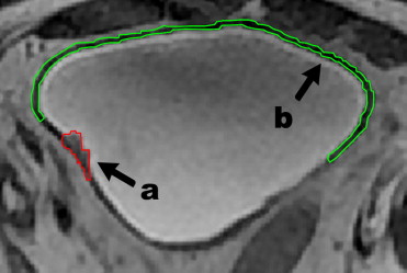
Regions of interest (ROIs) were manually placed on foci of bladder cancer and uninvolved bladder wall in 22 patients and on the normal bladder wall of 23 volunteers to calculate 40 known textural features. Statistical analysis was applied to determine the difference in these features in bladder cancer versus uninvolved bladder wall versus normal bladder wall of volunteers. The significantly different features were then analyzed using a support vector machine (SVM) classifier to determine their accuracy in differentiating malignancy from the bladder wall.
Results
Thirty-three of 40 features show significant differences between bladder cancer and the bladder wall. Nine of 40 features were significantly different in uninvolved bladder wall of patients versus normal bladder wall of volunteers. Further study indicates that seven of these 33 features were significantly different between uninvolved bladder wall of patients with early cancer and that of volunteers, whereas 15 of 33 features were different between that of patients with advanced cancer and normal wall. With the testing dataset consisting of ROIs acquired from patients, the classification accuracy using 33 textural features fed into the SVM classifier was 86.97%.
Conclusion
The initial experience demonstrates that texture features are sensitive to reveal the differences between bladder cancer and the bladder wall on MRI. The different features can be used to develop a computer-aided system for the evaluation of the entire bladder wall.
Bladder cancer is the fourth most common malignancy and accounts for 7% of all malignancies in men in the United States . In addition, according to the National Cancer Institute’s Surveillance Epidemiology and End Result Registry, there has been a rising trend in bladder cancer incidence by approximately 40% since 1975 . In China, bladder cancer is the ninth most common malignancy in men, with increasing incidence in areas with growing aging population or the worsening environment .
The recurrence of bladder cancer is very high and even early-stage bladder cancer is likely to recur. It is estimated that 50–70% of all diagnosed cases will recur and 10–30% will progress to muscularis invasive disease . For this reason, bladder cancer posses a significant economic burden, and survivors often undergo follow-up tests to look for bladder cancer recurrence for years after treatment. Therefore, early detection of bladder abnormalities in high-risk populations and an appropriate follow-up procedure for survivors in a convenient and noninvasive manner is crucial to prevent the disease and reduce the death rate.
Get Radiology Tree app to read full this article<
Get Radiology Tree app to read full this article<
Get Radiology Tree app to read full this article<
Materials and methods
Subjects
Get Radiology Tree app to read full this article<
Imaging Protocols
Get Radiology Tree app to read full this article<
Get Radiology Tree app to read full this article<
ROI Measurements
Get Radiology Tree app to read full this article<
Get Radiology Tree app to read full this article<
Get Radiology Tree app to read full this article<
Texture Analysis
Get Radiology Tree app to read full this article<
Get Radiology Tree app to read full this article<
Table 1a
The Textural Features Used in This Study (Simple Version)
Category N Features Distribution of image gray level 8 Mean, entropy, uniformity, SD, smoothness, skewness, Tm, kurtosis Auto-covariance coefficient 1 Norm of vector Tamura features 4 Contrast, directionality, line-likeness, regularity Features derived from GLCM 16 Sixteen features derived from the GLCM matrix, ie, f1: angular second moment, f2: contrast, f3: correlation, f4: sum of squares, f5: inverse difference moment, f6: sum average, f7: sum variance, f8: sum entropy, f9: entropy, f10: difference variance, f11: difference entropy, f12 and f13: information measures of correlation, f14: inertia, f15: cluster shade, and f16: cluster prominence. Features derived from GLGCM 11 Eleven features derived from the GLGCM matrix, ie, T1: small grads dominance, T2: big grads dominance, T3: gray asymmetry, T4: grads asymmetry, T5: energy, T6: correlation, T7: gray entropy, T8: grads entropy, T9: entropy. T10: inertia, and T11: DifferMoment.
Table 1b
The Textural Features Used in This Study (Version With Definitions)
Category Features Computation Formula Notes Distribution of image gray level Meanm=1n∑(x,y)∈R[f(x,y)] m
=
1
n
∑
(
x
,
y
)
∈
R
[
f
(
x
,
y
)
] f(x,y) represents the intensity value of a pixel located at ( x , y ). n means the total number of pixels within the ROI, k means the number of gray level value within the ROI, and p(l__i__) means the probability of value l__i occurring in the ROI. Entropye=−∑ki=1[p(li)]log2[p(li)] e
=
−
∑
i
=
1
k
[
p
(
l
i
)
]
log
2
[
p
(
l
i
)
] Uniformityu=∑ki=1[p(li)]2 u
=
∑
i
=
1
k
[
p
(
l
i
)
]
2 Standard deviations=1n−1∑ni=1[fi(x,y)−m)]2−−−−−−−−−−−−−−−−−−−−√ s
=
1
n
−
1
∑
i
=
1
n
[
f
i
(
x
,
y
)
−
m
)
]
2 SmoothnessR=1−11+s2 R
=
1
−
1
1
+
s
2 SkewnessS=n(n−1)(n−2)s3∑ni=1(li−m)3 S
=
n
(
n
−
1
)
(
n
−
2
)
s
3
∑
i
=
1
n
(
l
i
−
m
)
3 Third moment (Tm)μ3=∑ki=1(li−m)3p(li) μ
3
=
∑
i
=
1
k
(
l
i
−
m
)
3
p
(
l
i
) KurtosisK=n(n+1)(n−1)(n−2)(n−3)s4∑ni=1(li−m)4−3(n−1)2(n−2)(n−3) K
=
n
(
n
+
1
)
(
n
−
1
)
(
n
−
2
)
(
n
−
3
)
s
4
∑
i
=
1
n
(
l
i
−
m
)
4
−
3
(
n
−
1
)
2
(
n
−
2
)
(
n
−
3
) Auto-covariance coefficient Norm of vector (NOV)NOV=∑nΔm=0,Δn=0γ(Δm,Δn)2−−−−−−−−−−−−−−−−−−−−√ NOV
=
∑
Δ
m
=
0
,
Δ
n
=
0
n
γ
(
Δ
m
,
Δ
n
)
2 , where γ(Δm,Δn)=A(Δm,Δn)A(0,0) γ
(
Δ
m
,
Δ
n
)
=
A
(
Δ
m
,
Δ
n
)
A
(
0
,
0
) ,
A(Δm,Δn)=1Count(Δm,Δn)⋅∑M−1−Δmx=0∑N−1−Δny=0[fin(x,y)−f¯in]×[fin(x+Δm,y+Δn)−f¯in] A
(
Δ
m
,
Δ
n
)
=
1
C
o
u
n
t
(
Δ
m
,
Δ
n
)
·
∑
x
=
0
M
−
1
−
Δ
m
∑
y
=
0
N
−
1
−
Δ
n
[
f
i
n
(
x
,
y
)
−
f
¯
i
n
]
×
[
f
i
n
(
x
+
Δ
m
,
y
+
Δ
n
)
−
f
¯
i
n
] f in ( x, y ) and f in ( x+ Δ m, y+ Δ n ) are gray levels of pixels ( i , j ) and ( i +Δ m , j +Δ n ) inside a ROI of size M × N . f¯in f
¯
i
n is the mean value of all pixels and Count (Δ m, Δ n ) is the number of pixel pairs inside a ROI, with given distance (Δ m , Δ n ) along the x and y axes, respectively. Tamura features ContrastFcon=σ/(a4)1/4 F
c
o
n
=
σ
/
(
a
4
)
1
/
4 , where α4=μ4/σ4 α
4
=
μ
4
/
σ
4 μ__4 is the 4th moment of all pixels about the mean inside a ROI, and σ 2 is the variance. θ is the gradient direction of a pixel, and N θ ( k ) is the number of pixels with which (2k-1)π/2n < θ < (2k + 1)π/2n and the gradient norm |G| ≥ t (a preset thresholding). H__D ( ϕ ) can be regarded as the histogram of θ, where n__p is the number of peaks, ϕ__p is the position of the pth peak, and w__p is the range between peaks. P__Dd means the n x n local cooccurrence matrix with a given distance along a given direction. r is a normalizing factor and σ xxx means the standard deviation of the feature F__xxx . DirectionalityHD(k)=Nθ(k)/∑n−1i=0Nθ(i)k=0,1,⋯,n−1 H
D
(
k
)
=
N
θ
(
k
)
/
∑
i
=
0
n
−
1
N
θ
(
i
)
k
=
0
,
1
,
⋯
,
n
−
1
Fdir=∑npp∑ϕ∈wp(ϕ−ϕp)2HD(ϕ) F
d
i
r
=
∑
p
n
p
∑
ϕ
∈
w
p
(
ϕ
−
ϕ
p
)
2
H
D
(
ϕ
) Line-likenessFlin=∑ni∑njPDd(i,j)cos[(i−j)2πn]/∑ni∑njPDd(i,j) F
l
i
n
=
∑
i
n
∑
j
n
P
D
d
(
i
,
j
)
cos
[
(
i
−
j
)
2
π
n
]
/
∑
i
n
∑
j
n
P
D
d
(
i
,
j
) RegularityFreg=1−r(σcrs+σcon+σdir+σlin) F
r
e
g
=
1
−
r
(
σ
c
r
s
+
σ
c
o
n
+
σ
d
i
r
+
σ
l
i
n
)
where Fcrs=1M×N∑Mi=1∑Nj=1Sbest(i,j) F
c
r
s
=
1
M
×
N
∑
i
=
1
M
∑
j
=
1
N
S
b
e
s
t
(
i
,
j
) Features derived from GLCM f1–f16 derived from the GLCM matrixMd,θ(i,j)=∑Mx=1∑Ny=1{10if(x,y),(x′,y′)ɛR2,f(x,y)=iandf(x′,y′)=jotherwise M
d
,
θ
(
i
,
j
)
=
∑
x
=
1
M
∑
y
=
1
N
{
1
i
f
(
x
,
y
)
,
(
x
’
,
y
’
)
ɛ
R
2
,
f
(
x
,
y
)
=
i
a
n
d
f
(
x
’
,
y
’
)
=
j
0
o
t
h
e
r
w
i
s
e
f1: angular second moment, f2: contrast, f3: correlation, f4: sum of squares, f5: inverse difference moment, f6: sum average, f7: sum variance, f8: sum entropy, f9: entropy, f10: difference variance, f11: difference entropy, f12 &f13: information measures of correlation, f14: inertia, f15: cluster shade, and f16: cluster prominence.f ( x,y ) represents the intensity value of a pixel located at ( x , y ). M × N is the size of the ROI. M__d,θ ( i , j ) is the ( i , j ) element of the GLCM matrix, representing the relative frequency with which two pixels with given gray levels of i and j are separated by a given pixel distance of d along the direction of θ . Features derived from GLGCM T1–T11 derived from the GLGCM matrixM’(i,j)=∑Mx=1∑Ny=1{10if(x,y)ɛR2,f(x,y)=i and fg(x,y)=jotherwise M
’
(
i
,
j
)
=
∑
x
=
1
M
∑
y
=
1
N
{
1
if
(
x
,
y
)
ɛ
R
2
,
f
(
x
,
y
)
=
i and f
g
(
x
,
y
)
=
j
0
otherwise
T1: small grads dominance, T2: big grads dominance, T3: gray asymmetry, T4: grads asymmetry, T5: energy, T6: correlation, T7: gray entropy, T8: grads entropy, T9: entropy. T10: inertia, and T11: DifferMoment.f__g ( x,y ) represents the gradient image of f ( x , y ) . M’ ( i , j ) is the ( i , j ) element of the GLGCM matrix, representing the relative frequency with which a pixel with given gray level of i and gradient of j appeared in the ROI.
GLCM, gray level cooccurrence matrix; GLGCM, gray level-gradient cooccurrence matrix; grads, gradient; N, number of features; Tm, third moment.
Get Radiology Tree app to read full this article<
Get Radiology Tree app to read full this article<
Get Radiology Tree app to read full this article<
Initial Classification Using Selected Features
Get Radiology Tree app to read full this article<
Results
Get Radiology Tree app to read full this article<
Table 2
Histologic Subtypes and Staging of Patients
Subtype Stage Number Age Range Mean Age ± SD Uc T1 4 50–58 54.75 ± 3.59 Uc T2 13 32–73 59.31 ± 12.10 Uc T3 3 64–74 70.33 ± 5.50 Uc T4 2 66 66.00 ± 0.00 Total 22 32–74 60.59 ± 10.59
Uc, urothelial carcinoma.
Get Radiology Tree app to read full this article<
Get Radiology Tree app to read full this article<
Get Radiology Tree app to read full this article<
Table 3
t -test Results between Groups A and B (N a = 21, N b = 20)
Features_P_ (Two-Tailed) Features_P_ (Two-Tailed) Mean .0000 T9 .0000 Entropy .0000 T10 .0000 Uniformity .0010 T11 .0000 Standard deviation .0000 f1 .0000 Smoothness .0000 f2 .0000 Third movement .0000 f3 .0000 Norm .0000 f4 .0000 Contrast .0000 f5 .0000 Line_likeness .0060 f6 .0000 T1 .0000 f7 .0000 T2 .0000 f8 .0000 T3 .0000 f9 .0000 T4 .0080 f10 .0000 T5 .0010 f11 .0000 T7 .0000 f14 .0000 T8 .0098 f15 .0000 f16 .0000
The difference between groups A and B was considered to be significant if P < .01.
Get Radiology Tree app to read full this article<
Get Radiology Tree app to read full this article<
Table 4
t -test Results between Groups B and C (N b = 20, N c = 23)
Features_P_ (Two-tailed) Features_P_ (Two-tailed) Entropy .0000 T6 .0010 Uniformity .0000 T9 .0000 Directionality .0050 f1 .0000 T5 .0020 f9 .0000 f12 .0070
The difference between groups B and C was considered to be significant if P < .01.
Get Radiology Tree app to read full this article<
Get Radiology Tree app to read full this article<
Get Radiology Tree app to read full this article<
Table 5
Analysis of Variance between Groups B1 and C, B2 and C
Feature B2 and C_P_ B1 and C_P_ Mean ▵ .639 ○ .733 Entropy ▲ .001 ● .005 Uniformity ▲ .003 ● .011 Standard deviation ▲ .044 ○ .149 Smoothness ▵ .079 ○ .310 Third moment ▵ .362 ● .025 Norm ▵ .240 ○ .120 Contrast ▵ .138 ○ .176 Line_likeness ▲ .002 ○ .437 T1 ▵ .632 ○ .469 T2 ▵ .810 ○ .350 T3 ▲ .041 ○ .777 T4 ▲ .017 ○ .517 T5 ▲ .007 ● .014 T7 ▲ .042 ○ .856 T8 ▲ .021 ○ .218 T9 ▲ .000 ● .015 T10 ▵ .605 ○ .967 T11 ▵ .756 ○ .279 f1 ▲ .000 ● .005 f2 ▵ .186 ○ .814 f3 ▵ .931 ○ .134 f4 ▵ .565 ○ .453 f5 ▵ .085 ○ .861 f6 ▵ .736 ○ .681 f7 ▵ .603 ○ .672 f8 ▲ .007 ○ .753 f9 ▲ .000 ● .001 f10 ▲ .032 ○ .426 f11 ▲ .028 ○ .578 f14 ▵ .186 ○ .814 f15 ▵ .940 ○ .052 f16 ▵ .182 ○ .103
▲, significant difference between groups B2 and C; ▵, no significant difference between groups B2 and C; ●, significant difference between groups B1 and C; ○, no significant difference between groups B1 and C.
The difference between groups was considered to be significant if P < .05. Nine features show significant difference between subgroup B2 and group C and no significant difference between subgroup B1 and group C (indicated by ▲ and ○). Only one feature shows the opposite result (indicated by ▵ and ●).
Get Radiology Tree app to read full this article<
Get Radiology Tree app to read full this article<
Get Radiology Tree app to read full this article<
Discussion
Get Radiology Tree app to read full this article<
Get Radiology Tree app to read full this article<
Get Radiology Tree app to read full this article<
Get Radiology Tree app to read full this article<
Get Radiology Tree app to read full this article<
Get Radiology Tree app to read full this article<
Get Radiology Tree app to read full this article<
Acknowledgments
Get Radiology Tree app to read full this article<
Get Radiology Tree app to read full this article<
References
1. American Cancer Society : Cancer facts & figures 2012.2012.American Cancer SocietyAtlanta (GA)
2. Kirkali Z., Chan T., Murugesan M., et. al.: Bladder cancer: epidemiology, staging and grading, and diagnosis. Urology 2005; 66: pp. 4-34.
3. Bladder Cancer Clinical Guideline Update Panel : Bladder cancer: guideline for the management of nonmuscle invasive bladder cancer: (stages Ta, T1, and Tis): 2007 update.2007.American Urological AssociationLinthicum, MD
4. Committee of Chinese diagnosis and treatment guidelines in urology surgery : Chinese diagnosis and treatment guidelines in urology surgery.2007.China Urology Surgery Society
5. The top ten malignancy mortality rates of China (man) [EB/OL]. Available at: http://61.49.18.65/htmlfiles/zwgkzt/ptjnj/year2010/index2010.html . Accessed April 15, 2012.
6. Jacobs B.L., Lee C.T., Montie J.E.: Bladder cancer in 2010: how far have we come?. CA Cancer J Clin 2010; 60: pp. 244-272.
7. Kim J.K., Ahn J.H., Park T., et. al.: Virtual cystoscopy of the contrast material-filled bladder in patients with gross hematuria. AJR Am J Roentgenol 2002; 179: pp. 763-768.
8. Arslan H., Ceylan K., Harman M., et. al.: Virtual computed tomography cystoscopy in bladder pathologies. Clin Urol 2006; 32: pp. 147-154.
9. Sheshadri H.S., Kandaswamy A.: Experimental investigation on breast tissue classification based on statistical feature extraction of mammograms. Comp Med Imaging Graphics 2007; 31: pp. 46-48.
10. Ganeshan B., Miles K.A., Young R.C., et. al.: Texture analysis in non-contrast enhanced CT: impact of malignancy on texture in apparently disease-free areas of the liver. Eur J Radiol 2009; 70: pp. 101-110.
11. Totaro A., Pinto F., Brescia A., et. al.: Imaging in bladder cancer: present role and future perspectives. Urol Int 2010; 85: pp. 373-380.
12. Wu W.-J., Moon W.K.: Ultrasound breast tumor image computer-aided diagnosis with texture and morphological features. Acad Radiol 2008; 15: pp. 873-880.
13. Tamura H., Mori S., Yamawaki T.: Textural features corresponding to visual perception. IEEE Trans Syst Man Cybernetics 1978; 8: pp. 460-473.
14. Robert M.H., Shanmugam K., Dinstein I.: Textural features for image classification. IEEE Trans Syst Man Cybernetics 1973; SMC-3: pp. 610-621.
15. Conners R.W., Trivedi M.M., Harlow C.A.: Segmentation of a high-resolution urban scene using texture operators. Comp Vision Graphics Image Pro 1984; 25: pp. 273-310.
16. Scher A., Rosenfeld A.: “Probability transforms” of digital pictures. Pattern Recognit 1980; 12: pp. 457-468.
17. Nailon WH, Redpath AT, McLaren DB. Texture analysis of 3D bladder cancer CT images for improving radiotherapy planning. Paris, France: 13th International Power Electronics and Motion Control Conference; 2008;652–655.
18. National Comprehensive Cancer Network. NCCN Clinical Practice Guidelines in Oncology: Bladder Cancer VII. 2011. National Comprehensive Cancer Network; 2011.
19. Jaume S., Ferrant M., Macq B., et. al.: Tumor detection in the bladder wall with a measurement of abnormal thickness in CT scans. IEEE Trans Biomed Eng 2003; 50: pp. 383-390.
20. Reuter V.E.: The pathology of bladder cancer. Urology 2006; 67: pp. 11-18.
21. Lämmle M., Beer A., Settles M., et. al.: Reliability of MR imaging-based virtual cystoscopy in the diagnosis of cancer of the urinary bladder. AJR Am J Roentgenol 2002; 178: pp. 1483-1488.
22. Bernhardt T.M., Schmidl H., Philipp C., et. al.: Diagnostic potential of virtual cystoscopy of the bladder: MRI vs. CT – preliminary report. Eur Radiol 2003; 13: pp. 305-312.
23. Shi Z., Lu H., Wu Z., et. al.: Computer-aid detection and stage assessment of bladder cancer based on MR image. Int J CARS 2012; 7: pp. S275-S277.