Classification of Parenchymal Abnormality in Scleroderma Lung Using a Novel Approach to Denoise Images Collected via a Multicenter Study

Rationale and Objectives

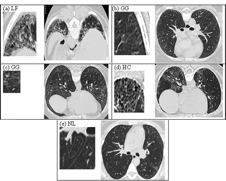
Computerized classification techniques have been developed to offer accurate and robust pattern recognition in interstitial lung disease using texture features. However, these techniques still present challenges when analyzing computed tomographic (CT) image data from multiprotocols because of disparate acquisition protocols or from standardized, multicenter clinical trials because of noise variability. Our objective is to investigate the utility of denoising thin section CT image data to improve the classification of scleroderma disease patterns. The patterns are lung fibrosis (LF), groundglass (GG), honeycomb (HC), or normal lung (NL) within small regions of interest (ROIs).

Methods

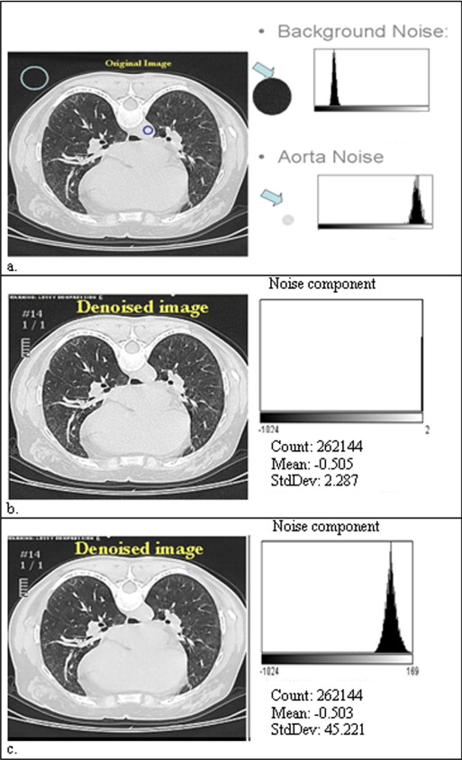
High-resolution CT images were scanned in a multicenter clinical trial for the Scleroderma Lung Study. A thoracic radiologist contoured a training set (38 patients) consisting of 148 ROIs with 46 LF, 85 GG, 4 HC, and 13 NL patterns and contoured a test set (33 new patients) consisting of 132 ROIs with 44 LF, 72 GG, 4 HC, and 12 NL patterns. The corresponding CT slices of a contoured ROI were denoised using Aujol’s mathematic partial differential equation algorithm. The algorithm’s noise parameter was estimated as the standard deviation of grey-level signal (in Hounsfield units) in a homogeneous, non-lung region: the aorta. Within each contoured ROI, every pixel within a 4 × 4 neighborhood was sampled (4 × 4 grid sampling). All sampled pixels from a contoured ROI were assumed to be the same disease pattern as labeled by the radiologist. 5,690 pixels (3,009 LF, 1,994 GG, 348 HC, and 339 NL) and 5,045 pixels (2,665 LF, 1,753 GG, 291 HC, and 336 NL) were sampled in training and test sets, respectively. Next, 58 texture features from the original and denoised image were calculated for each pixel. Using a multinomial logistic model, subsets of features (one from original and another from denoised images) were selected to classify disease patterns. Finally, pixels were classified into disease patterns using a support vector machine procedure.

Results

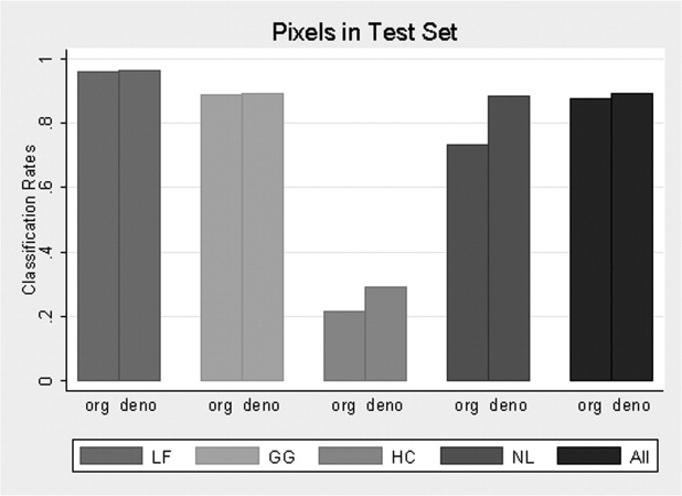
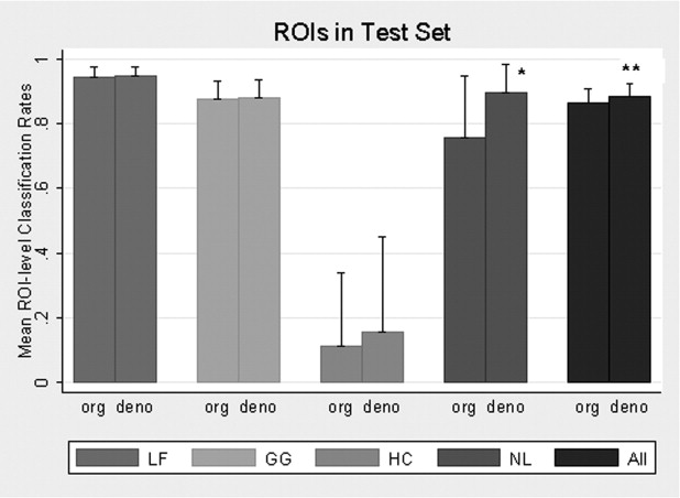
From the training set, multinomial logistic model selected 45 features from the original images and 38 features from denoised images to classify disease patterns. Using the test set, the overall pixel classification rate by SVM increased from 87.8% to 89.5% with denoising. The specific classification rates (original/denoised) were 96.3/96.4% for LF, 88.8/89.4% for GG, 21.3/28.9% for HC, and 73.5/88.4% for NL. Denoising significantly improved the NL and overall classification rates ( P = .037 and P = .047 respectively) at ROI level.

Conclusions

Analyzing multicenter data using a denoising approach led to more parsimonious classification models with increasing accuracy. This approach offers a novel alternate classification strategy for heterogeneous technical and disease components. Furthermore, the model offers the potential to discriminate the multiple patterns of scleroderma disease correctly.

There are no widely accepted classification techniques to score the extent of interstitial lung disease in multicenter trials ( ). It is especially important to offer an accurate and robust pattern classifier to help produce quantitative disease measures for both clinical care and research applications ( ). Although computer-generated texture features have been used to categorize interstitial lung disease patterns ( ), many challenges in their standardization prevent widespread use. Different radiation-dose protocols and disparate reconstruction kernels hamper the standardization process ( ).

Image noise is another factor that limits standardization, causing large variation in image quality. Image noise is affected by patient’s morphology, acquisition parameters, and computed tomographic (CT) platforms. Removing noise (denoising) has been shown to be clinically relevant to detect subtle abnormalities, such as groundglass (GG) opacity of the lung, and to decrease inter-reader variability ( ). Radiation dose may be increased to improve CT signaling, which reduces noise, but safety concerns restrict this procedure. Noise may only be removed by post-processing algorithms after the CT image is obtained.

Get Radiology Tree app to read full this article<

Materials and methods

Get Radiology Tree app to read full this article<

Image Denoising

Get Radiology Tree app to read full this article<

Scleroderma Lung Study

Get Radiology Tree app to read full this article<

Substudy Data

Get Radiology Tree app to read full this article<

Table 1

Summary of Training and Test Datasets

Numbers Patients Contoured ROIs Grid Sample Pixels Training set 38 148 (46 LF, 85 GG, 4 HC, 13 NL) 5,690 (3,009 LF, 1,994 GG, 348 HC, 339 NL) Test set 33 132 (44 LF, 72 GG, 4 HC, 12 NL) 5,045 (2,665 LF, 1,753 GG, 291 HC, 336 NL)

GG, groundglass; HC, honeycomb; LF, lung fibrosis; NL, normal lung; ROI, region of interest.

Get Radiology Tree app to read full this article<

Contouring

Get Radiology Tree app to read full this article<

Classification Procedures and Statistical Analyses

Get Radiology Tree app to read full this article<

Results

Get Radiology Tree app to read full this article<

Table 2

Test Set of Classification Result on ROI using Original Features with SVM Model for 4 Patterns: LF, GG, HC, and NL

Original Texture Feature Total LF GG HC NL True class LF 2,567 76 22 0 2,665 GG 184 1,556 0 13 1,753 HC 208 21 62 0 291 NL 0 89 0 247 336

GG, groundglass; HC, honeycomb; LF, lung fibrosis; NL, normal lung; ROI, region of interest; SVM, support vector machine.

Table 3

Test Set of Class Classification Result on Pixel using Denoised Features with SVM Model for 4 Patterns: LF, GG, HC, and NL

Denoised Texture Feature Total LF GG HC NL True class LF 2,569 72 24 0 2,665 GG 164 1,567 2 20 1,753 HC 198 7 84 2 291 NL 0 39 0 297 336

GG, groundglass; HC, honeycomb; LF, lung fibrosis; NL, normal lung; ROI, region of interest; SVM, support vector machine.

Get Radiology Tree app to read full this article<

Table 4

Test Set of Classification Result on ROI by Majority Vote for 4 Patterns: LF, GG, HC, and NL

Original Texture Feature Total LF GG HC NL True class by the radiologist LF 43 1 0 0 44 GG 6 66 0 0 72 HC 4 0 0 0 4 NL 0 2 0 10 12

GG, groundglass; HC, honeycomb; LF, lung fibrosis; NL, normal lung; ROI, region of interest; SVM, support vector machine.

Table 5

Test Set of Classification Result on ROI by Majority Vote for 4 Patterns: LF, GG, HC, and NL

Denoised Texture Feature Total LF GG HC NL True class by the radiologist LF 44 0 0 0 44 GG 5 67 0 0 72 HC 4 0 0 0 4 NL 0 0 0 12 12

GG, groundglass; HC, honeycomb; LF, lung fibrosis; NL, normal lung; ROI, region of interest; SVM, support vector machine.

Get Radiology Tree app to read full this article<

Discussion

Get Radiology Tree app to read full this article<

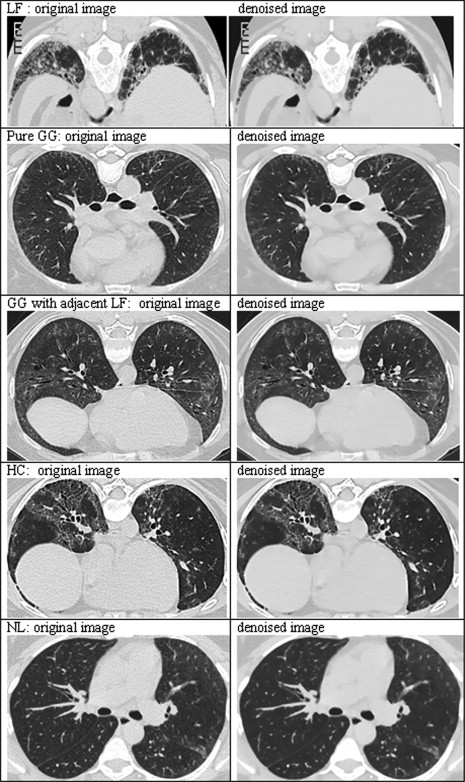
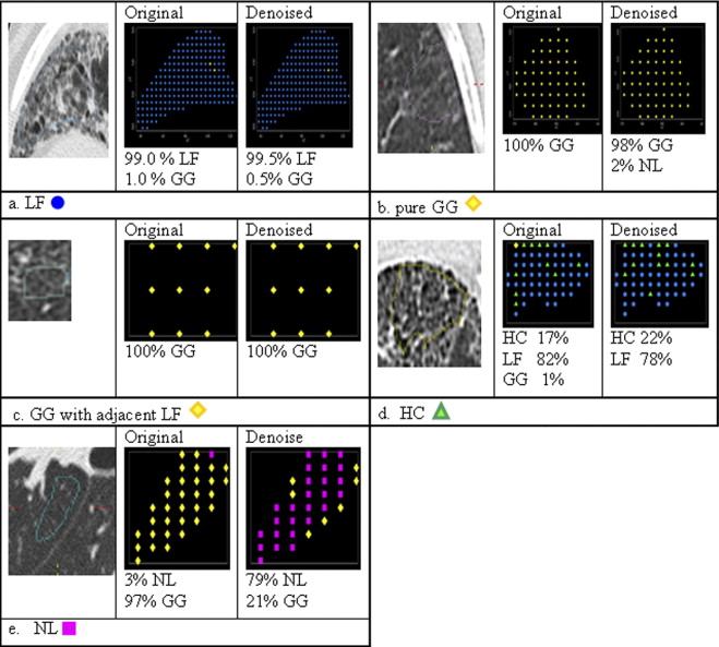
Principally, denoising reduced measurement error, permitting fewer features to classify disease types, and fewer features reduced bias associated with classification. NL classification improved the most ( Fig. 6 ); this observation meets expectations.

Get Radiology Tree app to read full this article<

Conclusion

Get Radiology Tree app to read full this article<

Acknowledgments

Get Radiology Tree app to read full this article<

Appendix 1 Modified Aujol’s Algorithm ( )

Get Radiology Tree app to read full this article<

1 Get Radiology Tree app to read full this article<

u0=0 u

Get Radiology Tree app to read full this article<

2 Get Radiology Tree app to read full this article<

wn+1=PδBG(f−un) w

n+1

(

−

)

un+1=f−wn+1−PλBG(f−wn+1) u

−

(

−

)

Get Radiology Tree app to read full this article<

3 Get Radiology Tree app to read full this article<

Get Radiology Tree app to read full this article<

max(|un+1−un|,|wn+1−wn|)≤ε, max

⁡

(

−

)

≤

where u and w represents the denoised and noised images, respectively, PBG P

G is a nonlinear projection described in Appendix 2 , and δ represents the amount of noise and λ represents the accuracy of the algorithm. The sum of u and w is approximately equal to the original CT image if the algorithm converges. Here, for the sake of simplicity, we set the noise parameter (δ) as 50, which was the upper bound of SD in the aorta across patients. Because the parameter has a certain threshold, the results of denoised images are similar to the values above the threshold. The residual parameter (λ) was set to 1, which controls the convergence of the algorithm.

Get Radiology Tree app to read full this article<

Appendix 2

Get Radiology Tree app to read full this article<

Projection

Get Radiology Tree app to read full this article<

p0=0 p

and

pn+1i,j=pni,j+τ(∇(div(pn)−f/λ))i,j1+τ∣∣(∇(div(pn)−f/λ))i,j∣∣. p

i,j

(

∇

(

div

(

)

−

)

i,j

(

∇

(

div

(

)

−

)

Theoretically, this projection converge τ ≤ 1/8. Practically, the author used 1/4 and he stated that it worked better ( ).

Get Radiology Tree app to read full this article<

Gradient Operator

Get Radiology Tree app to read full this article<

(∇u)1i,j={ui+1, j−ui, j0ifi<Nifi=N (

∇

)

i,j

{

i+1, j

−

i, j

and

(∇u)2i,j={ui,j+1−ui,j0ifj<Nifj=N. (

∇

)

{

−

Get Radiology Tree app to read full this article<

Divergence Operator

Get Radiology Tree app to read full this article<

(div(p))i,j=⎧⎩⎨⎪⎪⎪⎪p1i,j−p1i−1,jp1i,j−p1i−1,jif1<i<Nifi=1ifi=N+⎧⎩⎨⎪⎪⎪⎪p2i,j−p2i,j−1p2i,j−p2i,j−1if1<j<Nifj=1ifj=N. (

(

)

{

−

{

−

Get Radiology Tree app to read full this article<

References

1. Best A.C., Lynch A.M., Bozic C.M., et. al.: Quantitative CT indexes in idiopathic pulmonary fibrosis: relationship with physiologic impairment. Radiology 2003; 228: pp. 407-414.
2. Lynch D.A.: Quantitative CT of fibrotic interstitial lung disease. Chest 2007; 131: pp. 643-644.
3. Uppaluri R., Hoffman E.A., Sonka M., et. al.: Computer recognition of regional lung disease patterns. Am J Respir Crit Care Med 1999; 160: pp. 648-654.
4. Chabat F., Yang G.Z., Hansell D.M.: Obstructive lung diseases: texture classification for differentiation at CT. Radiology 2003; 228: pp. 871-877.
5. Kim K.G., Goo J.M., Kim J.H., et. al.: Computer-aided diagnosis of localized ground-glass opacity in the lung at CT: initial experience. Radiology 2005; 237: pp. 657-661.
6. Xu Y., van Beek E.J., Hwanjo Y., et. al.: Computer-aided classification of interstitial lung diseases via MDCT: 3D adaptive multiple feature method (3D AMFM). Acad Radiol 2006; 13: pp. 969-978.
7. Zavaletta V.A., Bartholmai B.J., Robb R.A.: High resolution multidetector CT-aided tissue analysis and quantification of lung fibrosis. Acad Radiol 2007; 14: pp. 772-787.
8. Abtin F., Goldin J.G., Suh R., et. al.: Denoising of HRCT images by statistical postprocessing image decomposition improves detection by ground glass opacities.2006. Oral Presentation, Scientific Session. RSNA, Nov 27, Chicago, IL
9. Donoho D.L., Johnstone I.: Adapting to unknown smoothness via wavelet shrinkage. J Am Stat Assoc 1995; 90: pp. 1200-1224.
10. Mallat S.G.: A wavelet tour of signal processing.1998.Academic PressSan Diego, CA
11. Rudin L.I., Osher S., Fatemi E.: Nonlinear total variation based noise removal algorithms. Physica D 1992; 60: pp. 259-268.
12. Nikolova M.: A variational approach to remove outliers and impulse noise. J Math Imaging Vision 2004; 20: pp. 99-120.
13. Aujol J.F., Gilboa G., Chan T., et. al.: Structure-texture image decomposition-modeling, algorithm, and parameter selection. Int J Comput Vision 2006; 67: pp. 111-136.
14. Yves Meyer: Oscillating patterns in image processing and in some nonlinear evolution equations. Vol 222001.American Mathematical SocietyProvidence, RI
15. Aujol J.F., Chambolle A.: Dual norm and image decomposition models. Int J Comput Vision 2005; 63: pp. 85-104.
16. Tashkin D.P., Elashoff R., Clements P.J., et. al.: Cyclophosphamide versus placebo in scleroderma lung disease. N Engl J Med 2006; 354: pp. 2655-2666.
17. Chambolle A.: An algorithm for total variation minimization and applications. J Math Imaging 2004; 20: pp. 89-97.
18. Sonka M., Hlavac V., Boyle R.: Image processing, analysis and machine vision.1993.Chapman & HallLondon, England
19. Haralick R.M., Shanmugam K.: Texture features for image classification. IEEE Trans Syst Man Cybernetics 1973; 3: pp. 610-621.
20. Scott Long J.: Regression models for categorical and limited dependent variables.1997.SageThousand Oaks, CA
21. Vapnik V.N.: The nature of statistical learning theory.1999.SpringerNew York
22. Maglogiannis I.G., Zafiropoulos E.P.: Characterization of digital medical images utilizing support vector machines. BMC Med Inform Decis Mak 2004; 4: pp. 4-32.
23. Chapelle O., Haffner P., Vapnik V.: Support vector machines for histogram based image classification. IEEE Trans Neural Networks 1999; 10: pp. 1055-1064.
24. Efron B., Tibshirani R.J.: An introduction to the bootstrap.1993.Chapman & HallBoca Raton, FL
25. McNitt-Gray M.: AAPM/RSNA physics tutorial for residents: topics in CT. Radiographics 2002; 22: pp. 1541-1553.
26. Kish L.: Survey sampling.1965.John Wiley & SonsNew York
27. Snijders T.A.B., Bosker R.J.: Standard errors and sample sizes for two-level research. J Ed Statis 1993; 18: pp. 237-259.
28. Lynch D.A., Travis W.D., Müller N.L., et. al.: Idiopathic interstitial pneumonias: CT features. Radiology 2005; 236: pp. 10-21.
29. Remy-Jardin M., Remy J., Giraud F., et. al.: Computed tomography assessment of ground-glass opacity: semiology and significance. J Thorac Imaging 1993; 8: pp. 249-264.
30. Webb W.R.: High resolution lung computed tomography. Radiol Clin N Am 1991; 29: pp. 1051-1063.
31. Brown M.S., Goldin J.G., Rogers S., et. al.: Computer-aided lung nodule detection in CT: results of large-scale observer test. Acad Radiol 2005; 12: pp. 681-686.

Classification of Parenchymal Abnormality in Scleroderma Lung Using a Novel Approach to Denoise Images Collected via a Multicenter Study

Rationale and Objectives

Methods

Results

Conclusions

Materials and methods

Image Denoising

Scleroderma Lung Study

Substudy Data

Contouring

Classification Procedures and Statistical Analyses

Results

Discussion

Conclusion

Acknowledgments

Appendix 1

Modified Aujol’s Algorithm ( )

Appendix 2

Projection

Gradient Operator

Divergence Operator

References

Further Reading

Abstracts of Funded National Institutes of Health Grants

Assessment of Pancreatic Tumor Resectability with Multidetector Computed Tomography

Computed Tomography–Navigated Transthoracic Core Biopsy of Pulmonary Lesions