Comparison of 1D, 2D, and 3D Nodule Sizing Methods by Radiologists for Spherical and Complex Nodules on Thoracic CT Phantom Images

Rationale and Objectives

To estimate and statistically compare the bias and variance of radiologists measuring the size of spherical and complex synthetic nodules.

Materials and Methods

This study did not require the institutional review board approval. Six radiologists estimated the size of 10 synthetic nodules embedded within an anthropomorphic thorax phantom from computed tomography scans at 0.8- and 5-mm slice thicknesses. The readers measured the nodule size using unidimensional (1D) longest in-slice dimension, bidimensional (2D) area from longest in-slice and longest perpendicular dimension, and three-dimensional (3D) semiautomated volume. Intercomparisons of bias (difference between average and true size) and variance among methods were performed after converting the 2D and 3D estimates to a compatible 1D scale.

Results

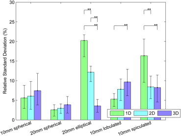
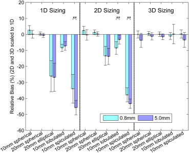
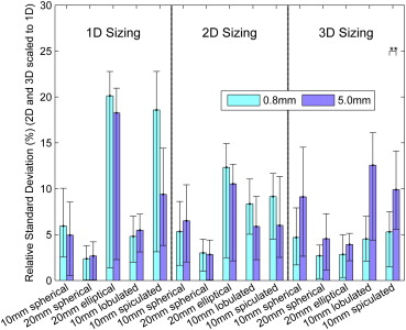
The relative biases of radiologists with the 3D tool were −1.8%, −0.4%, −0.7%, −0.4%, and −1.6% for 10-mm spherical, 20-mm spherical, 20-mm elliptical, 10-mm lobulated, and 10-mm spiculated nodules compared to 1.4%, −0.1%, −26.5%, −7.8%, and −39.8% for 1D. The three-dimensional measurements were significantly less biased than 1D for elliptical, lobulated, and spiculated nodules. The relative standard deviations for 3D were 7.5%, 3.9%, 3.6%, 9.7%, and 8.3% compared to 5.7%, 2.6%, 20.3%, 5.3%, and 16.4% for 1D. Unidimensional sizing was significantly less variable than 3D for the lobulated nodule and significantly more variable for the ellipsoid and spiculated nodules. Three-dimensional bias and variability were smaller for thin 0.8-mm slice data compared to thick 5.0-mm data.

Conclusions

The study shows that radiologist-controlled 3D volumetric lesion sizing can not only achieve smaller bias but also achieve similar or smaller variability compared to 1D sizing, especially for complex lesion shapes.

Multi-detector computed tomography (CT) imaging is a critical clinical tool in lung cancer evaluation. The recently reported results from the National Lung Screening Trial of subjects at high risk for lung cancer indicated that low-dose CT screening reduced lung cancer mortality by 20% compared to planar chest radiography screening . These results along with the results from the International Early Lung Cancer Action Program provide strong evidence that CT screening has potential as an effective tool for detecting early, more survivable lung cancers. CT imaging has also had an impact on the staging of lung cancers and is one of the factors that led to the updated guidelines on the TNM Classification of Malignant Tumors stage groupings in 2009 . Likewise, CT imaging has become a critically important tool for monitoring lung cancer patients undergoing therapy.

The response evaluation criteria in solid tumors (RECIST) is currently the quantitative standard used to assess disease progression in patients with lung cancer in clinical trials . Although it was originally developed for use only in clinical trials, clinicians routinely ask radiologists to provide RECIST measurements as an objective evaluation of patient response in daily practice . The measurement standard for tumor sizing used as part of RECIST is the longest, in-plane diameter of a tumor. This measurement standard, although simple to implement, is also problematic for complex cancers because tumors do not generally expand or contract uniformly . In an effort to address the limitations of RECIST and to potentially improve the sensitivity of the measurement to true anatomical changes, volumetric sizing has been proposed as an alternative quantitative approach for measuring anatomical changes in a lesion over time. However, questions have been raised as to whether volumetric analysis will add value or only increase the costs of patient care and the complexity of running clinical trials .

Get Radiology Tree app to read full this article<

Get Radiology Tree app to read full this article<

Get Radiology Tree app to read full this article<

Materials and methods

Get Radiology Tree app to read full this article<

Database Description

Get Radiology Tree app to read full this article<

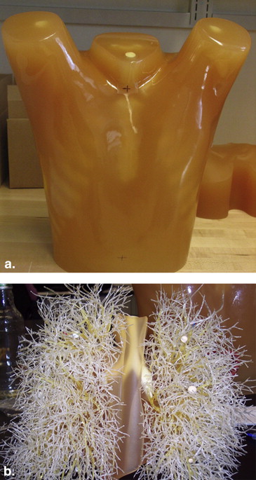
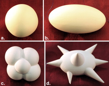
Table 1

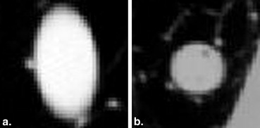
Technical Characteristics of the 10 Synthetic Nodules Evaluated (Five Nodules Shape/Size Combinations at Two Different X-ray Densities)

Shape Equivalent Diameter (mm) ∗ CT Densities Spherical 10 −10 HU, +100 HU Spherical 20 −10 HU, +100 HU Elliptical 20 −10 HU, +100 HU Lobulated 10 −10 HU, +100 HU Spiculated 10 −10 HU, +100 HU

CT, computed tomography; HU, Hounsfield units.

Get Radiology Tree app to read full this article<

Table 2

Scan Parameters Used in CT Data Acquisition

Acquisition Parameter Value Tube voltage 120 kVp Exposure 100 mAs/slice Pitch 1.2 Reconstructed slice thickness ∗ 0.8 mm (0.4 mm interval, 16 × 0.75 mm collimation) 5.0 mm (2.5 mm interval, 16 × 1.5 mm collimation) Reconstruction kernel Detail Repeat exposures 2 repeat scans of each nodule

CT, computed tomography.

Data acquired on a Philips 16-slice Mx8000 IDT scanner (Philips Healthcare, Andover, MA).

Get Radiology Tree app to read full this article<

Get Radiology Tree app to read full this article<

Reading Protocol

Get Radiology Tree app to read full this article<

Get Radiology Tree app to read full this article<

Get Radiology Tree app to read full this article<

Reference Standard

Get Radiology Tree app to read full this article<

VolumeNod=MassNodDensityNod V

o

l

u

m

e

N

o

d

=

M

a

s

s

N

o

d

D

e

n

s

i

t

y

N

o

d

Get Radiology Tree app to read full this article<

Statistical Methods

Get Radiology Tree app to read full this article<

PE1Size=Size1Est−Size1TrueSize1True×100%, P

E

S

i

z

e

1

=

S

i

z

e

E

s

t

1

−

S

i

z

e

T

r

u

e

1

S

i

z

e

T

r

u

e

1

×

100

%

,

PE2Size=Size2Est√−Size2True√Size2True√×100%, P

E

S

i

z

e

2

=

S

i

z

e

E

s

t

2

−

S

i

z

e

T

r

u

e

2

S

i

z

e

T

r

u

e

2

×

100

%

,

PE3Size=Size3Est√3−Size3True√3Size3True√3×100%, P

E

S

i

z

e

3

=

S

i

z

e

E

s

t

3

3

−

S

i

z

e

T

r

u

e

3

3

S

i

z

e

T

r

u

e

3

3

×

100

%

,

BiasiRel(PEiSize)=E[PEiSize]−0, and B

i

a

s

Re

l

i

(

P

E

S

i

z

e

i

)

=

E

[

P

E

S

i

z

e

i

]

−

0

, and

StdiRel(PEiSize)=Std(PEiSize). S

t

d

Re

l

i

(

P

E

S

i

z

e

i

)

=

S

t

d

(

P

E

S

i

z

e

i

)

.

where SizeiEst S

i

z

e

E

s

t

i , SizeiTrue S

i

z

e

T

r

u

e

i , and PEiSize P

E

S

i

z

e

i are the estimated size, reference standard size, and normalized error, respectively, for sizing method i ( i = 1, 2, 3 corresponds to the 1D, 2D, or 3D sizing method in equations (5) and (6)). The conversion of size to PE resulted in all PEiSize P

E

S

i

z

e

i estimates having a nominal zero bias as expressed in equation (5). All statistical comparisons were based on differences in relative bias or relative standard deviation.

Get Radiology Tree app to read full this article<

Get Radiology Tree app to read full this article<

Get Radiology Tree app to read full this article<

Get Radiology Tree app to read full this article<

Results

ANOVA and Goodness-of-Fit Analysis

Get Radiology Tree app to read full this article<

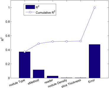
Table 3

ANOVA Table (One- and Two-Way Interactions) Limited to Nodule Type and Sizing Method as Fixed Factors (Ordered by Statistical Significance)

Source Sum of Squares d.f. Mean Squared Error F Probability > F Nodule type † 156362.9 4 39090.7 417.3 <.0001 Nodule type X sizing method † 81719 8 10214.9 109.1 <.0001 Sizing method † 49043.7 2 24521.8 261.8 <.0001 Unexplained error 133476 1425 93.7 Total 420601.6 1439

ANOVA, analysis of variance; d.f., degrees of freedom; F, F-statistic; X, denotes an interaction between terms.

Get Radiology Tree app to read full this article<

Get Radiology Tree app to read full this article<

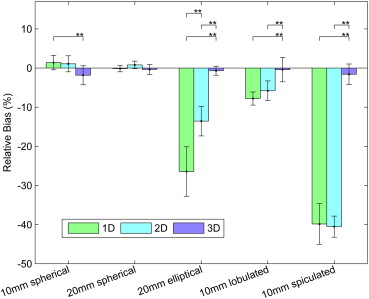
Comparison of Relative Bias among the Sizing Methods

Get Radiology Tree app to read full this article<

Table 4

Native and Relative Bias Estimates along with the Range in Relative Bias as a Function of Nodule Type and Sizing Method

Nodule Type Sizing Method Native Bias ∗ Relative Bias (%) Relative Bias Range (%) † 10-mm spherical 1D 0.14 1.41 −0.46, 3.27 2D 2.62 1.08 −0.97, 3.13 3D −18.87 −1.83 −4.26, 0.60 20-mm spherical 1D −0.02 −0.12 −0.97, 0.72 2D 6.98 0.81 −0.17, 1.78 3D −23.26 −0.35 −1.63, 0.93 20-mm elliptical 1D −8.42 −26.45 −32.79, −20.11 2D −121.23 −13.55 −17.34, −9.76 3D −70.38 −0.68 −1.84, 0.47 10-mm lobulated 1D −1.00 −7.79 −9.48, −6.11 2D −15.73 −5.8 −8.31, −3.29 3D 9.85 −0.4 −3.52, 2.72 10-mm spiculated 1D −9.04 −39.84 −45.03, −34.65 2D −217.55 −40.52 −43.22, −37.83 3D −13.44 −1.58 −4.19, 1.04

1D, unidimensional; 2D, bidimensional; 3D, three-dimensional.

Get Radiology Tree app to read full this article<

Get Radiology Tree app to read full this article<

Get Radiology Tree app to read full this article<

Comparison of Variability among the Sizing Methods

Get Radiology Tree app to read full this article<

Table 5

Native and Relative Variability as Defined by Standard Deviation along the Range in Variability as a Function of Nodule Type and Sizing Method

Nodule Type Sizing Method Native Standard ∗ Relative Standard (%) Relative Standard Range (%) † 10-mm spherical 1D 0.61 5.62 2.92, 8.84 2D 13.22 6.08 2.73, 9.82 3D 119.87 7.48 3.84, 11.88 20-mm spherical 1D 0.56 2.59 0.99, 3.88 2D 25.96 2.99 1.64, 4.08 3D 545.82 3.88 1.75, 5.99 20-mm elliptical 1D 6.59 20.25 16.11, 21.72 2D 109.03 12.18 9.76, 13.73 3D 480.08 3.58 1.97, 5.24 10-mm lobulated 1D 0.71 5.29 3.44, 6.73 2D 22.47 7.84 4.96, 10.47 3D 162.3 9.7 6.15, 12.95 10-mm spiculated 1D 3.90 16.36 9.60, 20.61 2D 35.53 8.4 5.39, 11.18 3D 131.01 8.26 4.58, 11.47

1D, unidimensional; 2D, bidimensional; 3D, three-dimensional.

Get Radiology Tree app to read full this article<

Get Radiology Tree app to read full this article<

Get Radiology Tree app to read full this article<

Comparison of Bias and Variability between Thin and Thick Slice CT Data

Get Radiology Tree app to read full this article<

Get Radiology Tree app to read full this article<

Repeatability of Reader Size Measurements

Get Radiology Tree app to read full this article<

Table 6

The Intra-Reader CCC as a Function of Sizing Method

Sizing Method CCC ∗ 1D 0.99 2D 0.99 3D 0.98

1D, unidimensional; 2D, bidimensional; 3D, three-dimensional; CCC, concordance correlation coefficient.

Get Radiology Tree app to read full this article<

Get Radiology Tree app to read full this article<

Discussion

Get Radiology Tree app to read full this article<

Get Radiology Tree app to read full this article<

Get Radiology Tree app to read full this article<

Get Radiology Tree app to read full this article<

Get Radiology Tree app to read full this article<

Get Radiology Tree app to read full this article<

Get Radiology Tree app to read full this article<

Get Radiology Tree app to read full this article<

Get Radiology Tree app to read full this article<

Get Radiology Tree app to read full this article<

Get Radiology Tree app to read full this article<

Acknowledgments

Get Radiology Tree app to read full this article<

Get Radiology Tree app to read full this article<

Get Radiology Tree app to read full this article<

References

• 1. National Lung Screening Trial Research Team, Aberle D.R., Adams A.M., Berg C.D., et. al.: Reduced lung-cancer mortality with low-dose computed tomographic screening. N Engl J Med 2011; 365: pp. 395-409.

• 2. International Early Lung Cancer Action Program Investigators, Henschke C.I., Yankelevitz D.F., Libby D.M., et. al.: Survival of patients with stage I lung cancer detected on CT screening. [see comment] N Engl J Med 2006; 355: pp. 1763-1771.

• 3. Buckler A.J., Mulshine J.L., Gottlieb R., et. al.: The use of volumetric CT as an imaging biomarker in lung cancer. Acad Radiol 2010; 17: pp. 100-106.

• 4. Goldstraw P.: The 7th Edition of TNM in Lung Cancer: what now?. J Thorac Oncol 2009; 4: pp. 671-673.

• 5. Goldstraw P., Crowley J., Chansky K., et. al.: The IASLC Lung Cancer Staging Project: proposals for the revision of the TNM stage groupings in the forthcoming (seventh) edition of the TNM Classification of malignant tumours. [Erratum appears in J Thorac Oncol. 2007 Oct;2(10):985] J Thorac Oncol 2007; 2: pp. 706-714.

• 6. Mozley P.D., Schwartz L.H., Bendtsen C., et. al.: Change in lung tumor volume as a biomarker of treatment response: a critical review of the evidence. Ann Oncol 2010; 21: pp. 1751-1755.

• 7. Eisenhauer E.A., Therasse P., Bogaerts J., et. al.: New response evaluation criteria in solid tumours: revised RECIST guideline (version 1.1). Eur J Cancer 2009; 45: pp. 228-247.

• 8. Suzuki C., Jacobsson H., Hatschek T., et. al.: Radiologic measurements of tumor response to treatment: practical approaches and limitations. Radiographics 2008; 28: pp. 329-344.

• 9. Gavrielides M.A., Kinnard L.M., Myers K.J., et. al.: Noncalcified lung nodules: volumetric assessment with thoracic CT. Radiology 2009; 251: pp. 26-37.

• 10. Zhao B., James L.P., Moskowitz C.S., et. al.: Evaluating variability in tumor measurements from same-day repeat CT scans of patients with non-small cell lung cancer. Radiology 2009; 252: pp. 263-272.

• 11. Zhao B., Schwartz L.H., Moskowitz C.S., et. al.: Lung cancer: computerized quantification of tumor response—initial results. Radiology 2006; 241: pp. 892-898.

• 12. Chen B., Barnhart H., Richard S., et. al.: Quantitative CT: technique dependence of volume estimation on pulmonary nodules. Phys Med Biol 2012; 57: pp. 1335-1348.

• 13. Das M., Ley-Zaporozhan J., Gietema H.A., et. al.: Accuracy of automated volumetry of pulmonary nodules across different multislice CT scanners. Eur Radiol 2007; 17: pp. 1979-1984.

• 14. Tran L.N., Brown M.S., Goldin J.G., et. al.: Comparison of treatment response classifications between unidimensional, bidimensional, and volumetric measurements of metastatic lung lesions on chest computed tomography. Acad Radiol 2004; 11: pp. 1355-1360.

• 15. Ko J.P., Rusinek H., Jacobs E.L., et. al.: Small pulmonary nodules: volume measurement at chest CT—phantom study. Radiology 2003; 228: pp. 864-870.

• 16. Brandman S., Ko J.P.: Pulmonary nodule detection, characterization, and management with multidetector computed tomography. J Thorac Imaging 2011; 26: pp. 90-105.

• 17. de Hoop B., Gietema H., van Ginneken B., et. al.: A comparison of six software packages for evaluation of solid lung nodules using semi-automated volumetry: what is the minimum increase in size to detect growth in repeated CT examinations. Eur Radiol 2009; 19: pp. 800-808.

• 18. Gavrielides M.A., Zeng R., Myers K.J., et. al.: Benefit of overlapping reconstruction for improving the quantitative assessment of CT lung nodule volume. Acad Radiol 2013; 20: pp. 173-180.

• 19. Quantitative Imaging Biomarkers Alliance. Radiological Society of North America (RSNA); 2010. Available at: www.rsna.org/research/qiba.cfm . Accessed October 23, 2013.

• 20. Petrick N., Kim H.J.G., Clunie D., et. al.: Evaluation of 1D, 2D and 3D nodule size estimation by radiologists for spherical and non-spherical nodules through CT thoracic phantom imaging.Summers R.M.van Ginneken B.SPIE Medical Imaging.2011.SPIELake Buena Vista, Florida, USA: 79630D1–7963D7

• 21. Gavrielides M.A., Kinnard L.M., Myers K.J., et. al.: A resource for the development of methodologies for lung nodule size estimation: database of thoracic CT scans of an anthropomorphic phantom. Opt Express 2010; 18: pp. 15244-15255.

• 22. World Health Organization: WHO handbook for reporting results of cancer treatment.1979.World Health OrganisationGeneva, Switzerland

• 23. Jolly M.P., Grady L.: 3D general lesion segmentation in CT. Proc IEEE Int Symp Biomed Imaging 2008; pp. 796-799.

• 24. Grady L.: Random walks for image segmentation. IEEE Trans Pattern Anal Mach Intell 2006; 28: pp. 1768-1783.

• 25. Altman D.G.: Practical statistics for medical research.1991.Chapman and Hall/CRC PressBoca Raton, FL

• 26. Lin L.I.: A concordance correlation coefficient to evaluate reproducibility. Biometrics 1989; 45: pp. 255-268.