
Rationale and Objectives
Flat lesions in the colon may result in false-negative computed tomography colonography interpretations. It is unknown whether flat lesions are better measured on two-dimensional (2D) or three-dimensional (3D) images and which settings are optimal for enhanced reproducibility and decreased variability. We evaluated these factors to determine whether 2D or 3D is best for flat lesion measurements.
Methods and Materials
Eighty-eight lesions in 66 patients from a previously published clinical trial were analyzed. Lesions were viewed with four methods including 2D at three window/level settings and 3D endoluminal view. Lesions in either supine or prone were counted as one dataset. Long axis and height were measured. Criteria of “height” (≤3 mm high) or “ratio” (height ≤half the long axis) were applied. A subset of lesions was subject to inter- and intra-observer variability analysis.
Results
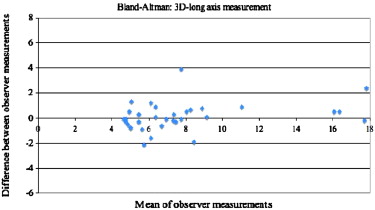
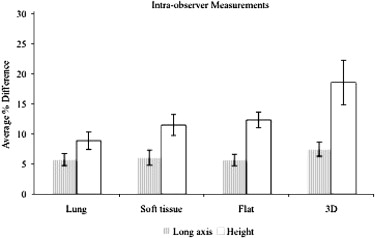
With the “height” criterion, more datasets were classified as flat in 2D flat ( n = 76), 2D soft tissue ( n = 82), and 3D ( n = 73) views than in the 2D lung ( n = 49) view. If long axis is used as the key metric, endoluminal 3D (12.1%) views significantly showed the least inter-observer variability compared to lung (18.9%) or soft tissue (20.2%) views. Intra-observer variability was low overall for all methods.
Conclusion
When characterizing lesions as flat, a consistent viewing method should be used. To minimize inter-observer variability (such as when following a patient over time), it is best to use the ratio criterion for flat lesion definition incorporating the single longest dimension on 3D views as the key metric.
Flat lesions of the colon are a potentially important source of false negative computed tomography colonography (CTC) interpretations . Several different definitions of flat lesions have been proposed including height <3 mm, a definition recommended in a consensus opinion and a height less than one-half the width (as seen on two-dimensional [2D] views, or long axis as seen on three-dimensional [3D] views). In many CTC investigations and clinical reports, endoscopists and radiologists may classify a lesion as “flat” based on subjective visual impression without defining the term in their methods or without measuring the lesion .
There are no clinical data to indicate whether flat lesions are better measured on 2D views or the 3D endoluminal views. On 2D views, the optimal window and level settings to visualize or to measure a flat lesion have not been determined.
Get Radiology Tree app to read full this article<
Materials and methods
Study Population
Get Radiology Tree app to read full this article<
Observers
Get Radiology Tree app to read full this article<
Lesion Assessment
Get Radiology Tree app to read full this article<
Get Radiology Tree app to read full this article<
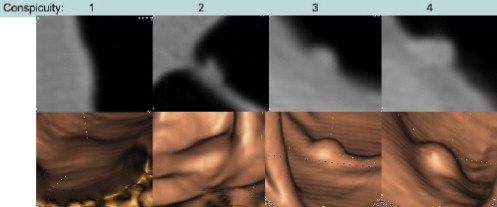
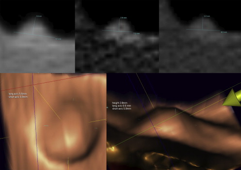
Lesion Conspicuity and Measurement
Get Radiology Tree app to read full this article<
Statistical Experimental Design
Get Radiology Tree app to read full this article<
Intra-observer Variability
Get Radiology Tree app to read full this article<
Inter-observer Variability
Get Radiology Tree app to read full this article<
Results
Definition
Get Radiology Tree app to read full this article<
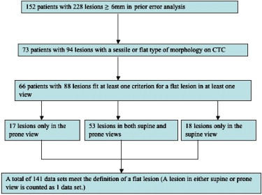
Table 1
OC, Long Axis, and Height Measurements in the Two-dimensional Lung View Comparing 68 Adenomas (121 Datasets) versus 26 Non-adenomas (39 Datasets)
Adenoma ( n = 68) Non-adenoma ( n = 26) Mean (mm) Standard Deviation Mean (mm) Standard Deviation OC 8.83 3.08 7.48 1.78 Long axis 9.09 2.93 8.26 2.46 Height 3.81 1.32 3.28 0.65
OC, optical colonoscopy; CTC, computed tomography colonography.
One dataset was not visualized in the two-dimensional lung view. Ninety-four lesions (161 datasets) in 73 patients seen on CTC had flat or sessile type morphologies that were measured to determine if they fit a proposed flat lesion definition. Non-adenomas included those classified as normal, hyperplastic, or other. A lesion in either supine or prone view is counted as one dataset. OC measurements ranged from 6–18 mm in size.
Get Radiology Tree app to read full this article<
Get Radiology Tree app to read full this article<
Table 2
The Number of Datasets that Fit Two Different Definitions of a Flat Lesion
2D Lung 2D Soft Tissue 2D Flat 3D_n_ = 141n = 134n = 135n = 141 Fits less than or equal to 3 mm height definition (% of total) 49 (34.8%) 82 (61.2%) 76 (56.3%) 73 (51.8%) Fits height less than half the longest axis definition (% of total) 116 (82.3%) 110 (82.1%) 121 (89.6%) 119 (84.4%)
2D, two-dimensional; 3D, three-dimensional.
Seven and six datasets could not be visualized in the 2D soft tissue and flat views, respectively.
Get Radiology Tree app to read full this article<
Conspicuity
Get Radiology Tree app to read full this article<
Comparison of Viewing Methods
Get Radiology Tree app to read full this article<
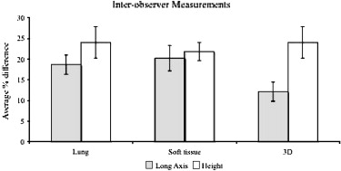
Table 3
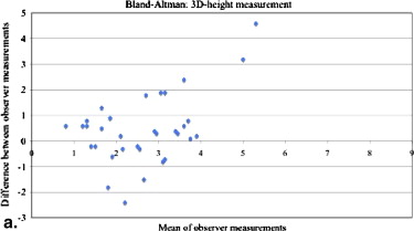
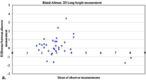
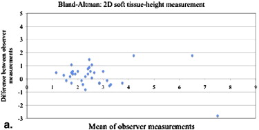
Statistical Analysis of Height Measurements Taken by Observer #1 Compared to Observer #2 in the 2D Lung, 2D Soft Tissue, and 3D Endoluminal Views
Measurement Parameter Mean Percentage Difference (%) ∗ Mean Difference (mm) † Standard Deviation of Difference 95% Bland-Altman Limits of Agreement ‡ 2D Lung 24.1 0.26 1.07 -1.84, 2.36 2D soft tissue 21.8 0.26 0.84 -1.39, 1.91 3D 24.1 0.47 1.36 -2.21, 3.14
2D, two-dimensional; 3D, three-dimensional.
Get Radiology Tree app to read full this article<
Get Radiology Tree app to read full this article<
Get Radiology Tree app to read full this article<
Table 4
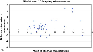
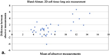
Statistical Analysis of Long Axis Measurements Taken by Observer #1 Compared to Observer #2 in the 2D Lung, 2D Soft Tissue, and 3D Endoluminal Views
Measurement Parameter Mean Percentage Difference (%) ∗ Mean Difference (mm) † Standard Deviation of Difference 95% Bland-Altman Limits of Agreement ‡ 2D Lung 18.9 0.94 2.32 -3.61,5.48 2D soft tissue 20.2 0.92 2.22 -3.43, 5.28 3D 12.1 0.46 2.11 -3.67, 4.59
2D, two-dimensional; 3D, three-dimensional.
Get Radiology Tree app to read full this article<
Get Radiology Tree app to read full this article<
Get Radiology Tree app to read full this article<
Get Radiology Tree app to read full this article<
Lesion Measurements
Get Radiology Tree app to read full this article<
Get Radiology Tree app to read full this article<
Discussion
Definition
Get Radiology Tree app to read full this article<
Comparison of Viewing Methods
Get Radiology Tree app to read full this article<
Conspicuity and Measurement
Get Radiology Tree app to read full this article<
Lesion Follow-up
Get Radiology Tree app to read full this article<
Source of Variability
Get Radiology Tree app to read full this article<
Get Radiology Tree app to read full this article<
Get Radiology Tree app to read full this article<
Acknowledgments
Get Radiology Tree app to read full this article<
Appendix 1
Get Radiology Tree app to read full this article<
Get Radiology Tree app to read full this article<
Get Radiology Tree app to read full this article<
References
1. Fidler J.L., Johnson C.D., MacCarty R.L., et. al.: Detection of flat lesions in the colon with CT colonography. Abdom Imaging 2002; 27: pp. 292-300.
2. Park S.H., Ha H.K., Kim A.Y., et. al.: Flat polyps of the colon: detection with 16-MDCT colonography—preliminary results. AJR Am J Roentgenol 2006; 186: pp. 1611-1617.
3. Sawada T., Hojo K., Moriya Y.: Colonoscopic management of focal and early colorectal carcinoma. Balliere Clin Gastroenterol 1989; 3: pp. 627-645.
4. Kudo S., Kashida H., Tamura T., et. al.: Colonoscopic diagnosis and management of nonpolypoid early colorectal cancer. World J Surg 2000; 24: pp. 1081-1090.
5. The Paris endoscopic classification of superficial neoplastic lesions: esophagus, stomach, and colon. Gastrointest Endosc 2003; 58: pp. S3-S43.
6. Soetikno R., Friedland S., Kaltenbach T., et. al.: Gastroenterology 2006; 130: pp. 566-576.
7. Pickhardt P.J., Nugent P.A., Choi J.R., et. al.: Flat colorectal lesions in asymptomatic adults: implications for screening with CT virtual colonoscopy. AJR Am J Roentgenol 2004; 183: pp. 1343-1347.
8. Endoscopic Classification Review Group: Update on the Paris classification of superficial neoplastic lesions in the digestive tract. Endoscopy 2005; 37: pp. 570-578.
9. The Paris endoscopic classification of superficial neoplastic lesions: esophagus, stomach, and colon: November 30 to December 1, 2002. Gastrointest Endosc 2003; 58: pp. S3-S43.
10. Zalis M.E., Barish M.A., Choi J.R., et. al.: Working Group on Virtual Colonoscopy. CT colonography reporting and data system: a consensus proposal. Radiology 2005; 236: pp. 3-9.
11. Kim D.H., Pickhardt P.J., Taylor A.J., et. al.: CT colonography versus colonoscopy for the detection of advanced neoplasia. N Engl J Med 2007; 357: pp. 1403-1412.
12. Rockey D., Paulson E., Niedzwiecki D., et. al.: Analysis of air contrast barium enema, computed tomographic colonography, and colonoscopy: prospective comparison. Lancet 2005; 365: pp. 305-311.
13. Doshi T., Rusinak D., Halvorsen R.A., et. al.: CT colonography: false-negative interpretations. Radiology 2007; 244: pp. 165-173.
14. Park S.H., Lee S.S., Choi E.K., et. al.: Flat colorectal neoplasms: definition, importance, and visualization on CT colonography. Zalis ME, Barish MA, Choi JR, et al. Working Group on Virtual Colonoscopy 2007; 188: pp. 953-959.
15. Pickhardt P.J., Choi J.R., Hwang I., et. al.: Computed tomographic virtual colonoscopy to screen for colorectal neoplasia in asymptomatic adults. N Engl J Med 2003; 349: pp. 191-200.
16. Young B.M., Fletcher J.G., Paulsen S.R., et. al.: Polyp measurement with CT colonography: multiple-reader, multiple-workstation comparison. AJR Am J Roentgenol 2007; pp. 122-129.
17. Summers R.M., Frentz S.M., Liu J., et. al.: Conspicuity of colorectal polyps at CT colonography: visual assessment, CAD performance, and the important role of polyp height. Acad Radiol 2009; 16: pp. 4-14.