Computer-aided Assessment of Regional Abdominal Fat with Food Residue Removal in CT

Rationale and Objectives

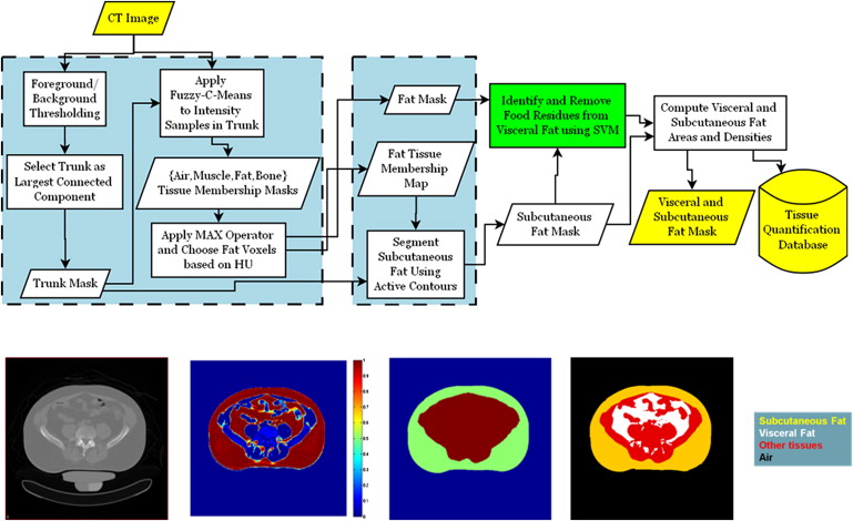
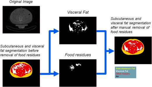
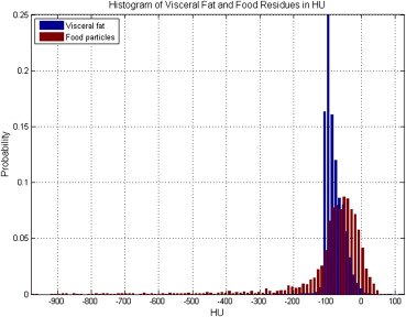
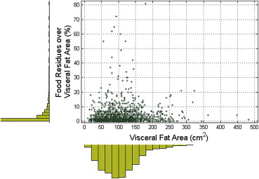
Separate quantification of abdominal subcutaneous and visceral fat regions is essential to understand the role of regional adiposity as risk factor in epidemiological studies. Fat quantification is often based on computed tomography (CT) because fat density is distinct from other tissue densities in the abdomen. However, the presence of intestinal food residues with densities similar to fat may reduce fat quantification accuracy. We introduce an abdominal fat quantification method in CT with interest in food residue removal.

Materials and Methods

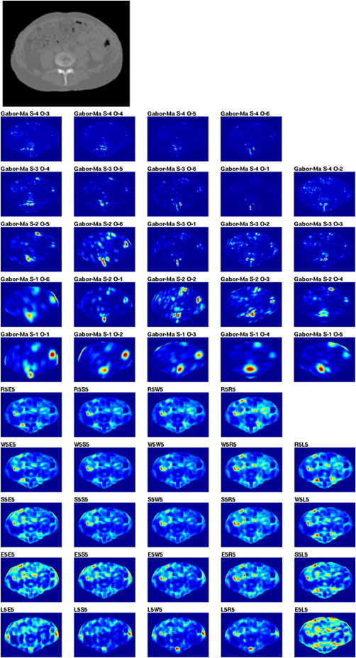
Total fat was identified in the feature space of Hounsfield units and divided into subcutaneous and visceral components using model-based segmentation. Regions of food residues were identified and removed from visceral fat using a machine learning method integrating intensity, texture, and spatial information. Cost-weighting and bagging techniques were investigated to address class imbalance.

Results

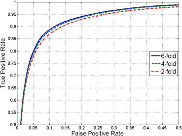
We validated our automated food residue removal technique against semimanual quantifications. Our feature selection experiments indicated that joint intensity and texture features produce the highest classification accuracy at 95%. We explored generalization capability using k -fold cross-validation and receiver operating characteristic (ROC) analysis with variable k . Losses in accuracy and area under ROC curve between maximum and minimum k were limited to 0.1% and 0.3%. We validated tissue segmentation against reference semimanual delineations. The Dice similarity scores were as high as 93.1 for subcutaneous fat and 85.6 for visceral fat.

Conclusions

Computer-aided regional abdominal fat quantification is a reliable computational tool for large-scale epidemiological studies. Our proposed intestinal food residue reduction scheme is an original contribution of this work. Validation experiments indicate very good accuracy and generalization capability.

Abdominal obesity is strongly related to metabolic disorders, hypertension, and cardiovascular disease . Separate quantification of visceral and subcutaneous fat in the abdomen is important because of their different metabolic consequences and because visceral fat more than subcutaneous fat has been associated with numerous age-related problems, such as insulin resistance, chronic inflammation, and cardiac diastolic dysfunction. Computed tomography (CT) is a widely adopted technique for assessing abdominal fat. Measurements of subcutaneous and visceral fat areas are typically computed from CT images using manual or semimanual analyses operated by clinical specialists. Even though these techniques usually provide reliable results, they are time-consuming and affected by intra- and inter-operator variability. Therefore, a regional fat quantification approach is highly desirable to increase the analysis throughput and reproducibility, especially in large epidemiological studies .

Earlier abdomen fat quantification approaches required user intervention to define a region of interest and detected the fat voxels using density thresholding techniques in the domain of Hounsfield units (HUs). More recent techniques make use of joint intensity and texture information in a fuzzy affinity framework to identify the fat class , employ shape and appearance models for quantification of regional fat and muscle compartments , or use radial analysis to delineate the boundary between subcutaneous and visceral fat .

Get Radiology Tree app to read full this article<

Materials and methods

Get Radiology Tree app to read full this article<

Participants and CT Imaging

Get Radiology Tree app to read full this article<

Subcutaneous and Visceral Fat Segmentation

Get Radiology Tree app to read full this article<

Removal of Food Residues

Get Radiology Tree app to read full this article<

Feature Analysis

Get Radiology Tree app to read full this article<

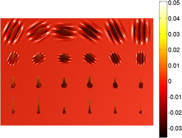
G(x,y)=12πσxσye[−12(x2σ2x+y2σ2y)+j2πWx] G

(

)

[

−

(

)

]

Get Radiology Tree app to read full this article<

Classification Using SVMs

Get Radiology Tree app to read full this article<

L(w,b,a)=12w2−∑Nn=1an{tn(wTφ(xn)+b)−1} L

(

)

−

∑

{

(

)

−

}

where a = { a__1 ,… a__N }. For nonlinear decision functions, the solution is to define a kernel function K(xi,xj)=φ(xi),φ(xj) K

(

)

(

)

(

) . Advantages of this technique are good generalization capability, robustness in high dimensions, and convexity of the objective function. Because of these advantages, the literature of SVM theory and applications is very broad. More detailed and formal descriptions of SVMs can be found elsewhere .

Get Radiology Tree app to read full this article<

Modeling for Imbalanced Classification

Get Radiology Tree app to read full this article<

Results

Get Radiology Tree app to read full this article<

Table 1

Comparison of Different Feature Computation and Selection Schemes

Feature Domain D TPR (%) TNR (%) ACC (%) AUC I, S, G, L, LS, NLS 63 97.6 ± 0.3 65.8 ± 3.8 95.0 ± 0.5 0.954 I, S, G, L, NLS 58 97.5 ± 0.3 65.5 ± 3.9 95.0 ± 0.5 0.953 I, S, G, L, LS 58 97.5 ± 0.3 65.4 ± 3.9 94.9 ± 0.7 0.953 I, S, G, L 53 97.5 ± 0.4 63.9 ± 4.4 94.7 ± 0.6 0.950 I, S, G 29 94.2 ± 1.0 73.3 ± 2.8 92.6 ± 1.0 0.941 I, S, L 29 93.5 ± 1.0 80.0 ± 3.4 92.4 ± 1.0 0.946 I, S 5 85.0 ± 1.8 84.9 ± 4.4 85.0 ± 1.5 0.923 I 3 69.5 ± 2.9 81.7 ± 2.4 70.5 ± 2.5 0.846 HDR-based 44 97.1 ± 0.8 68.5 ± 9.3 94.8 ± 0.6 0.953 Fisher-based 30 93.1 ± 1.2 80.1 ± 3.9 92.0 ± 1.1 0.943 PCA 25 96.7 ± 0.5 68.4 ± 4.2 94.4 ± 0.6 0.949

ACC, classification accuracy; AUC, area under the receiver operating characteristic curve; Fisher, Fisher’s distance ranking; G, Gabor features; HDR, hierarchical dimensionality reduction; I, intensity features; L, Law’s features; LS, linear scale-space; NLS, nonlinear scale-space; PCA, principal component analysis; S, spatial coordinates; TNR, true-negative rate; TPR, true-positive rate.

Get Radiology Tree app to read full this article<

Table 2

Classification Rates and AUC of k -fold Cross-Validation Experiment for k∈{2,4,6} k

∈

{

} Using All Computed Features ( D = 63)

k -fold TPR (%) TNR (%) ACC (%) AUC 2 97.8 ± 0.2 61.3 ± 0.6 94.9 ± 0.5 0.951 4 97.6 ± 0.9 64.7 ± 0.3 94.9 ± 0.7 0.952 6 97.6 ± 0.3 65.8 ± 3.8 95.0 ± 0.5 0.954

ACC, classification accuracy; AUC, area under the receiver operating characteristic curve; TNR, true-negative rate; TPR, true-positive rate.

Get Radiology Tree app to read full this article<

Table 3

Classification Rates and (AUC) of k -fold Cross-Validation with Repeated Undersampling and Bagging for k∈{2,4,6} k

∈

{

} Using All Computed Features ( D = 63)

k -fold TPR (%) TNR (%) ACC (%) AUC 2 95.7 ± 0.5 74.6 ± 0.7 94.0 ± 0.7 0.951 4 95.7 ± 0.6 75.9 ± 2.4 94.1 ± 0.8 0.953 6 95.8 ± 0.8 76.4 ± 6.8 94.2 ± 0.6 0.953

ACC, classification accuracy; AUC, area under the receiver operating characteristic curve; TNR, true-negative rate; TPR, true-positive rate.

Get Radiology Tree app to read full this article<

Table 4

Segmentation Validation for Subcutaneous Fat, Visceral Cavity, and Visceral Fat

Subcutaneous Region Visceral Cavity Visceral Fat Pearson correlation coefficient (ρ 2 ) 0.983 0.993 0.956 Relative area error (%) 5.4 ± 4.5 1.7 ± 1.1 8.2 ± 8.8 Dice coefficient (%) 93.1 ± 2.9 98.4 ± 5.5 85.6 ± 5.7

Get Radiology Tree app to read full this article<

Discussion

Get Radiology Tree app to read full this article<

Acknowledgments

Get Radiology Tree app to read full this article<

References

1. Kissebah A.H., Vydelingum N., Murray R., et. al.: Relation of body fat distribution to metabolic complications of obesity. J Clin Endocrinol Metabol 1982; 54: pp. 254-260.
2. Seidell J.C., Hautvast J.G., Deurenberg P.: Overweight: fat distribution and health risks. Epidemiological observations. a review. Infusionstherapie 1989; 16: pp. 276-281.
3. Beydoun M.A., Lhotsky A., Wang Y., et. al.: Association of adiposity status and changes in early to mid-adulthood with incidence of Alzheimer’s disease. Am J Epidemiol 2008; 168: pp. 1179-1189.
4. Ding J., Kritchevsky S.B., Hsu F.-C., et. al.: Association between non-subcutaneous adiposity and calcified coronary plaque: a substudy of the multi-ethnic study of atherosclerosis. Am J Clin Nutr 2008; 88: pp. 645-650.
5. Lee K., Lee S., Kim Y., et. al.: Waist circumference, dual-energy X-ray absortiometrically measured abdominal adiposity, and computed tomographically derived intra-abdominal fat area on detecting metabolic risk factors in obese women. Nutrition 2008; 24: pp. 625-631.
6. Kanaya A.M., Lindquist K., Harris T.B., et. al.: Total and regional adiposity and cognitive change in older adults: the health, aging and body composition (ABC) study. Arch Neurol 2009; 66: pp. 329-335.
7. Jensen M.D., Kanaley J.A., Reed J.E., et. al.: Measurement of abdominal and visceral fat with computed tomography and dual-energy x-ray absorptiometry. Am J Clin Nutr 1995; 61: pp. 274-278.
8. Yoshizumi T., Nakamura T., Yamane M., et. al.: Abdominal fat: standardized technique for measurement at CT. Radiology 1999; 211: pp. 283-286.
9. Bandekar A., Naghavi M., Kakadiaris I.: Performance evaluation of abdominal fat burden quantification in CT. Conf Proc IEEE Eng Med Biol Soc 2005; 3: pp. 3280-3283.
10. Chung H., Cobzas D., Birdsell L., et. al.: Automated segmentation of muscle and adipose tissue on CT images for human body composition analysis. Proc SPIE 2009; 7261: 72610K
11. Zhao B., Colville J., Kalaigian J., et. al.: Automated quantification of body fat distribution on volumetric computed tomography. J Comput Assist Tomogr 2006; 30: pp. 777-783.
12. Bezdek J.C.: Pattern recognition with fuzzy objective function algorithms.1981.Kluwer Academic PublishersNorwell, MA
13. Xu C., Prince J.L.: Snakes, shapes, and gradient vector flow. IEEE Trans Image Proc 1998; 7: pp. 359-369.
14. Unser M., Aldroubi A.: A review of wavelets in biomedical applications. Proc IEEE 1996; 84: pp. 626-638.
15. Daugman J.: Complete discrete 2-D Gabor transforms by neural networks for image analysis and compression. IEEE Trans Acoustics. Speech Signal Proc 1988; 36: pp. 1169-1179.
16. Manjunath B., Ma W.: Texture features for browsing and retrieval of image data. IEEE Trans Pattern Anal Machine Intell 1996; 18: pp. 837-842.
17. Lee T.S.: Image representation using 2D Gabor wavelets. IEEE Trans Pattern Anal Machine Intell 1996; 18: pp. 959-971.
18. Shapiro L.G., Stockman G.C.: Computer vision.2001.Prentice Hall
19. Iijima T.: Basic theory on normalization of a pattern (in case of typical one-dimensional pattern). Bull Electrical Lab 1962; 26: pp. 368-388. [in Japanese]
20. Witkin A.: Scale-space filtering. Int Jt Conf Artificial Intell 1983; pp. 1019-1022.
21. Koenderink J.J.: The structure of images. Biol Cybernetics 1984; 50: pp. 363-370.
22. Makrogiannis S., Vanhamel I., Fotopoulos S., et. al.: A watershed-based multiscale segmentation method for color images using automatic scale selection. SPIE J Electronic Imaging 2005; pp. 14.
23. Alpert N.M., Bradshaw J.F., Kennedy D., et. al.: The principal axes transformation–a method for image registration. J Nucl Med 1990; 31: pp. 1717-1722.
24. Arata L.K., Dhawan A.P., Broderick J.P., et. al.: Three-dimensional anatomical model-based segmentation of MR brain images through Principal Axes Registration. IEEE Trans Biomed Eng 1995; 42: pp. 1069-1078.
25. Duda R.O., Hart P.E., Stork D.G.: Pattern classification.2000.Wiley-Interscience Publication
26. Burges C.J.C.: A tutorial on support vector machines for pattern recognition. Data Min Knowl Discovery 1998; 2: pp. 121-167.
27. Cortes C., Vapnik V.: Support-vector networks. Mach Learn 1995; 20: pp. 273-297.
28. Chang CC, Lin CJ. LIBSVM: a library for support vector machines 2006. Software available at: http://www.csie.ntu.edu.tw/∼cjlin/libsvm .
29. Tang Y., Zhang Y.Q., Chawla N.V., et. al.: SVMs modeling for highly imbalanced classification. IEEE Trans Syst Man Cybernetics, Part B: Cybernetics 2009; 39: pp. 281-288.
30. Dice L.R.: Measures of the amount of ecologic association between species. Ecology 1945; 26: pp. 297-302.

Computer-aided Assessment of Regional Abdominal Fat with Food Residue Removal in CT

Rationale and Objectives

Materials and Methods

Results

Conclusions

Materials and methods

Participants and CT Imaging

Subcutaneous and Visceral Fat Segmentation

Removal of Food Residues

Feature Analysis

Classification Using SVMs

Modeling for Imbalanced Classification

Results

Discussion

Acknowledgments

References

Further Reading

Accuracy of Axillary Lymph Node Staging in Breast Cancer Patients

Accurate Detection of Metabolically Active “Brown” and “White” Adipose Tissues with Computed Tomography

Analysis of Dominant Factors Affecting Fatigue Caused by Soft-Copy Reading