Computer-aided Diagnosis for Lung Cancer

Rationale and Objectives

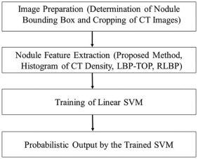
To develop a computer-aided diagnosis system to differentiate between malignant and benign nodules.

Materials and Methods

Seventy-three lung nodules revealed on 60 sets of computed tomography (CT) images were analyzed. Contrast-enhanced CT was performed in 46 CT examinations. The images were provided by the LUNGx Challenge, and the ground truth of the lung nodules was unavailable; a surrogate ground truth was, therefore, constructed by radiological evaluation. Our proposed method involved novel patch-based feature extraction using principal component analysis, image convolution, and pooling operations. This method was compared to three other systems for the extraction of nodule features: histogram of CT density, local binary pattern on three orthogonal planes, and three-dimensional random local binary pattern. The probabilistic outputs of the systems and surrogate ground truth were analyzed using receiver operating characteristic analysis and area under the curve. The LUNGx Challenge team also calculated the area under the curve of our proposed method based on the actual ground truth of their dataset.

Results

Based on the surrogate ground truth, the areas under the curve were as follows: histogram of CT density, 0.640; local binary pattern on three orthogonal planes, 0.688; three-dimensional random local binary pattern, 0.725; and the proposed method, 0.837. Based on the actual ground truth, the area under the curve of the proposed method was 0.81.

Conclusions

The proposed method could capture discriminative characteristics of lung nodules and was useful for the differentiation between malignant and benign nodules.

Introduction

In the United States, it was projected that 1,665,540 new cancer cases and 585,720 cancer deaths would occur in 2014, with 86,930 male and 72,330 female Americans dying from lung cancer . Lung cancer is the leading cause of cancer deaths. For most cancers, there have been notable improvements in survival rates over the past three decades, but lung and pancreatic cancers have shown the least improvement .

Computed tomography (CT) has high sensitivity in detecting lung nodules and improves the likelihood of detecting lung cancer at an early stage. However, it can be difficult for a radiologist or a pulmonologist to differentiate between malignant and benign lung nodules on CT. For example, in the National Lung Screening Trial, the rate of positive results was 24.2% with low-dose helical CT screening over all three rounds, and a total of 96.4% of the positive results in the low-dose CT group were false positives . False-positive findings can result in unnecessary follow-up CT scans, positron emission tomography scans, and invasive procedures such as bronchoscopy or surgical resection, raising concerns about the increased radiation or surgery risks for the patient .

Get Radiology Tree app to read full this article<

Materials and Methods

Get Radiology Tree app to read full this article<

CT Images

Get Radiology Tree app to read full this article<

Evaluation by Radiologists and Construction of Surrogate Ground Truth

Get Radiology Tree app to read full this article<

Computer-aided Diagnosis

Get Radiology Tree app to read full this article<

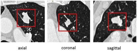
Image Preparation

Get Radiology Tree app to read full this article<

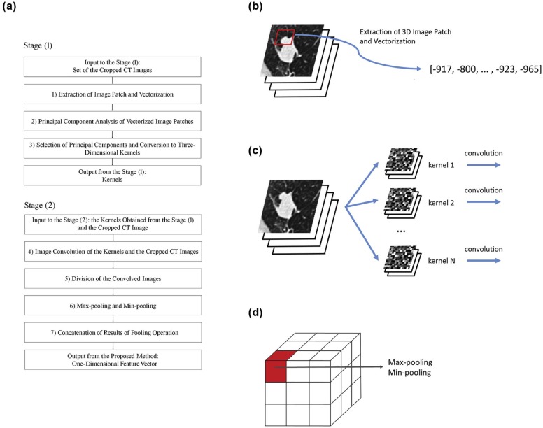
The Proposed CADx Method

Get Radiology Tree app to read full this article<

X=[x1,x2,…,xM], X

[

…

]

where x i ( i = 1… M ) denotes the vectorized image patch and is represented as a column vector. Next, the covariance matrix Y = XX T was obtained, and PCA was performed by calculating the eigenvalues and eigenvectors of Y . From the results of the PCA, N principal components (each with length R 3 ) were selected, corresponding to the 1st … N th largest absolute eigenvalues of Y . Then, the N principal components were converted to N 3D kernels in the reverse way to the vectorization of the 3D image patches. Here, the 3D kernel is denoted by W j ( j = 1… N ).

Get Radiology Tree app to read full this article<

Jij=Ii⊗Wj, J

⊗

where ⊗ ⊗ denotes 3D image convolution. Before image convolution, the boundary of I i was zero padded.

Get Radiology Tree app to read full this article<

fijk=maxx∈SijkJij(x) f

max

∈

(

)

gijk=minx∈SijkJij(x) g

min

∈

(

)

ri=[fi11,gi11,…,fi1K,gi1K,fi21,gi21,…,fi2K,gi2K,…,fiN1,giN1,…,fiNK,giNK], r

[

…

]

where J ij (x) is the value of J ij at the voxel x . In the proposed method, r i is the nodule feature of I i , and used for classification of the lung nodule revealed on I i .

Get Radiology Tree app to read full this article<

Other Methods

Get Radiology Tree app to read full this article<

LBP(x,Rl,Pl)=∑Pl−1i=02i×s(di)di=I(n(x,Rl,i))−I(x), L

(

)

∑

−

(

)

(

)

−

(

)

where x is the center pixel where LBP is calculated; P l is the number of samples; R l is the radius; n ( x, R l , i ) is the i th neighbor pixel around the center pixel x , and the distance between the center pixel x and the neighbor pixel is R l ; I ( u ) is the CT density of pixel u ; and s ( v ) is an indicator function, where s ( v ) is 1 if v ≥ 0 and 0 otherwise. To use LBP in 3D CT images, LBP-TOP was employed for the current study . In LBP-TOP, 2D LBP was calculated on the XY, XZ, and YZ planes, and the texture information on other 3D planes was ignored. Then, the results of 2D LBP on the XY, XZ, and YZ planes were converted into histograms, and the three histograms were concatenated, resulting in a 1D vector as a nodule feature.

Get Radiology Tree app to read full this article<

yi=pi−I(x), y

−

(

)

where yi y

i and pi p

i are the i th elements of vectors y and p , respectively. Sets of random vectors w j ( j = 1 … L r , L r is a predefined parameter) are selected, where each element of the random vector is uniformly distributed in [−1,1] and the length of w j is L r . The feature vector f for voxel “ x ” is obtained by using the following formula:

hj=s(wj⋅y) h

(

⋅

)

f=[h1,h2,…,hLr], f

[

…

]

where s () is the indicator function. In the previous study, f was evaluated by voxel-by-voxel analysis. In the current study, the nodule feature g is calculated as follows:

g=[∑xh1Nr,∑xh2Nr,…,∑xhLrNr], g

[

∑

…

∑

]

where N r is the number of voxels included in 3D CT images I . The nodule feature g is represented as a 1D vector with length L r , and used for the CADx system.

Get Radiology Tree app to read full this article<

Machine Learning

Get Radiology Tree app to read full this article<

Parameters

Get Radiology Tree app to read full this article<

Statistical Analysis

Get Radiology Tree app to read full this article<

Additional Evaluation

Get Radiology Tree app to read full this article<

Results

Get Radiology Tree app to read full this article<

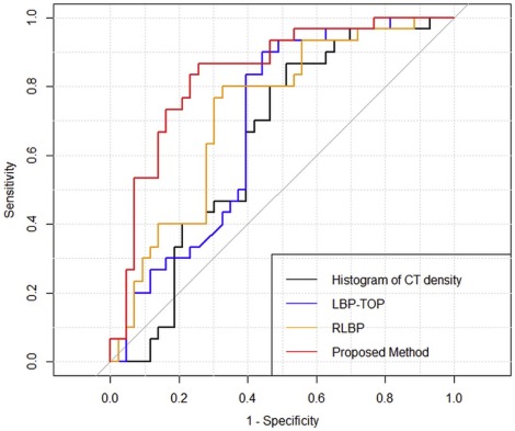
TABLE 1

Results of ROC Analysis of the CADx Systems

Method Sensitivity Specificity AUC Histogram of CT density 0.867 0.488 0.640 LBP-TOP 0.900 0.558 0.688 RLBP 0.800 0.674 0.725 Proposed method 0.867 0.744 0.837

AUC, area under the curve; CADx, computer-aided diagnosis for classification; CT, computed tomography; LBP-TOP, local binary pattern on three orthogonal planes; RLBP, three-dimensional random local binary pattern; ROC, receiver operating characteristic.

Note: Sensitivity and specificity were obtained at the optimal cutoff of the ROC curve.

TABLE 2

Results of DeLong Tests of AUC and NRI and IDI of the Reclassification Table Between the Proposed Method and the Three Other Methods

Method DeLong Test Categorical NRI IDI_P_ Value_P_ Value_P_ Value Histogram of CT density vs. proposed method .0059 <.0001 <.0001 LBP-TOP vs. proposed method .0176 .0002 .0007 RLBP vs. proposed method .135 .0045 .0060

AUC, area under the curve; CT, computed tomography; IDI, integrated discrimination improvement; LBP-TOP, local binary pattern on three orthogonal planes; NRI, net reclassification improvement; RLBP, three-dimensional random local binary pattern.

Note: Categorical NRI was calculated by grouping the probabilistic outputs into four categories (0–0.25, 0.25–0.5, 0.5–0.75, and 0.75–1).

Get Radiology Tree app to read full this article<

Discussion

Get Radiology Tree app to read full this article<

Conclusions

Get Radiology Tree app to read full this article<

Acknowledgments

Get Radiology Tree app to read full this article<

Supplementary Data

Get Radiology Tree app to read full this article<

Figure S1

Get Radiology Tree app to read full this article<

Figure S2

Get Radiology Tree app to read full this article<

Table S1

Get Radiology Tree app to read full this article<

Table S2

Get Radiology Tree app to read full this article<

Table S3

Get Radiology Tree app to read full this article<

Table S4

Get Radiology Tree app to read full this article<

Table S5

Get Radiology Tree app to read full this article<

Appendix S1

Get Radiology Tree app to read full this article<

References

1. Siegel R., Ma J., Zou Z., et. al.: Cancer statistics, 2014. CA Cancer J Clin 2014; 64: pp. 9-29.
2. National Lung Screening Trial Research Team, Aberle D.R., Adams A.M., et. al.: Reduced lung-cancer mortality with low-dose computed tomographic screening. N Engl J Med 2011; 65: pp. 395-409.
3. Aberle D.R., Abtin F., Brown K.: Computed tomography screening for lung cancer: has it finally arrived? Implications of the National Lung Screening Trial. J Clin Oncol 2013; 31: pp. 1002-1008.
4. Suzuki K.: A review of computer-aided diagnosis in thoracic and colonic imaging. Quant Imaging Med Surg 2012; 2: pp. 163-176.
5. Lee S.L.A., Kouzani A.Z., Hu E.J.: Automated detection of lung nodules in computed tomography images: a review. Mach Vis Appl 2012; 23: pp. 151-163.
6. El-Baz A., Beache G.M., Gimel’farb G., et. al.: Computer-aided diagnosis systems for lung cancer: challenges and methodologies. Int J Biomed Imaging 2013; 2013: pp. 942353.
7. Matsuki Y., Nakamura K., Watanabe H., et. al.: Usefulness of an artificial neural network for differentiating benign from malignant pulmonary nodules on high-resolution CT: evaluation with receiver operating characteristic analysis. AJR Am J Roentgenol 2002; 178: pp. 657-663.
8. Way T., Chan H.P., Hadjiiski L., et. al.: Computer-aided diagnosis of lung nodules on CT scans: ROC study of its effect on radiologists’ performance. Acad Radiol 2010; 17: pp. 323-332.
9. Way T.W., Hadjiiski L.M., Sahiner B., et. al.: Computer-aided diagnosis of pulmonary nodules on CT scans: segmentation and classification using 3D active contours. Med Phys 2006; 33: pp. 2323-2337.
10. Aoyama M., Li Q., Katsuragawa S., et. al.: Computerized scheme for determination of the likelihood measure of malignancy for pulmonary nodules on low-dose CT images. Med Phys 2003; 30: pp. 387-394.
11. Li F., Li Q., Engelmann R., et. al.: Improving radiologists’ recommendations with computer-aided diagnosis for management of small nodules detected by CT. Acad Radiol 2006; 13: pp. 943-950.
12. Arai K., Herdiyeni Y., Okumura H.: Comparison of 2D and 3D local binary pattern in lung cancer diagnosis. Int J Adv Comput Sci Appl 2012; 3: pp. 89-95.
13. Awai K., Murao K., Ozawa A., et. al.: Pulmonary nodules: estimation of malignancy at thin-section helical CT effect of computer-aided diagnosis on performance of radiologists. Radiology 2006; 239: pp. 276-284.
14. Chen H., Xu Y., Ma Y., et. al.: Neural network ensemble-based computer-aided diagnosis for differentiation of lung nodules on CT images: clinical evaluation. Acad Radiol 2010; 17: pp. 595-602.
15. Li Z., Yu L., Trzasko J.D., et. al.: Adaptive nonlocal means filtering based on local noise level for CT denoising. Med Phys 2014; 41: pp. 011908.
16. Liao S., Gao Y., Lian J., et. al.: Sparse patch-based label propagation for accurate prostate localization in CT images. IEEE Trans Med Imaging 2013; 32: pp. 419-434.
17. Tong T., Wolz R., Gao Q., et. al.: Multiple instance learning for classification of dementia in brain MRI. Med Image Comput Comput Assist Interv 2013; 16: pp. 599-606.
18. Armato S.G., Hadjiiski L., Tourassi G.D., et. al.: Guest editorial: LUNGx challenge for computerized lung nodule classification: reflections and lessons learned. J Med Imaging 2015; 2: pp. 020103.
19. Ojala T., Pietikäinen M., Harwood D.: A comparative study of texture measures with classification based on feature distributions. Pattern Recognit 1996; 29: pp. 51-59.
20. Ojala T., Pietikäinen M., Mäenpää T.: Multiresolution gray-scale and rotation invariant texture classification with local binary patterns. IEEE Trans Pattern Anal Mach Intell 2002; 24: pp. 971-987.
21. Zhao G., Pietikäinen M.: Dynamic texture recognition using local binary patterns with an application to facial expressions. IEEE Trans Pattern Anal Mach Intell 2007; 29: pp. 915-928.
22. Zhu H., Cheng H., Fan Y.: Random local binary pattern based label learning for multi-atlas segmentation. Proceedings of SPIE 9413, medical imaging 2015: image processing. Vol. 94131B2015. March 20, 2015
23. Labusch K., Barth E., Martinetz T.: Simple method for high-performance digit recognition based on sparse coding. IEEE Trans Neural Netw 2008; 19: pp. 1985-1989.
24. Chang C.C., Lin C.J.: LIBSVM: a library for support vector machines. ACM Trans Intell Syst Technol 2011; 2: pp. 1-27.
25. DeLong E.R., DeLong D.M., Clarke-Pearson D.L.: Comparing the areas under two or more correlated receiver operating characteristic curves: a nonparametric approach. Biometrics 1988; 44: pp. 837-845.
26. Pencina M.J., D’Agostino R.B., D’Agostino R.B., et. al.: Evaluating the added predictive ability of a new marker: from area under the ROC curve to reclassification and beyond. Stat Med 2008; 27: pp. 157-172.
27. Kundu S., Aulchenko Y.S., van Duijn C.M., et. al.: PredictABEL: an R package for the assessment of risk prediction models. Eur J Epidemiol 2011; 26: pp. 261-264.
28. Robin X., Turck N., Hainard A., et. al.: pROC: an open-source package for R and S+ to analyze and compare ROC curves. BMC Bioinformatics 2011; 12: pp. 77.
29. Guyon I., Weston J., Barnhill S., et. al.: Gene selection for cancer classification using support vector machines. Mach Learn 2002; 46: pp. 389-422.
30. Kamiya A., Murayama S., Kamiya H., et. al.: Kurtosis and skewness assessments of solid lung nodule density histograms: differentiating malignant from benign nodules on CT. Jpn J Radiol 2014; 32: pp. 14-21.
31. Aerts H.J., Velazquez E.R., Leijenaar R.T., et. al.: Decoding tumour phenotype by noninvasive imaging using a quantitative radiomics approach. Nat Commun 2014; 5: pp. 4006.
32. Chicklore S., Goh V., Siddique M., et. al.: Quantifying tumour heterogeneity in 18F-FDG PET/CT imaging by texture analysis. Eur J Nucl Med Mol Imaging 2013; 40: pp. 133-140.
33. Tetko I.V., Livingstone D.J., Luik A.I.: Neural network studies. 1. Comparison of overfitting and overtraining. J Chem Inf Comput Sci 1995; 35: pp. 826-833.
34. Velazquez E.R., Parmar C., Jermoumi M., et. al.: Volumetric CT-based segmentation of NSCLC using 3D-Slicer. Sci Rep 2013; 3: pp. 3529.

Computer-aided Diagnosis for Lung Cancer

Rationale and Objectives

Materials and Methods

Results

Conclusions

Introduction

Materials and Methods

CT Images

Evaluation by Radiologists and Construction of Surrogate Ground Truth

Computer-aided Diagnosis

Image Preparation

The Proposed CADx Method

Other Methods

Machine Learning

Parameters

Statistical Analysis

Additional Evaluation

Results

Discussion

Conclusions

Acknowledgments

Supplementary Data

References

Further Reading

Addition of the Fleischner Society Guidelines to Chest CT Examination Interpretive Reports Improves Adherence to Recommended Follow-up Care for Incidental Pulmonary Nodules

Analog Method for Radiographic Assessment of Heterotopic Bone in Fibrodysplasia Ossificans Progressiva

Another Time, Another Space