
Rationale and Objectives
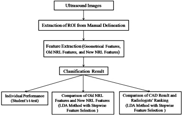
The aim of this study was to develop a semi-automated computer-aided diagnosis (CAD) system based on high-resolution ultrasonography for classifying benign and malignant soft tissue tumors (STTs).
Materials and Methods
One hundred seven patients with STTs (70 benign and 37 malignant) were enrolled, and regions of interest were manually delineated for analysis. Sixteen tumor shape features, including five geometric features and 11 morphologic features (six old and five new normalized radial length [NRL] features) were individually evaluated using Student’s t test and the area under the receiver-operating characteristic curve ( A z ). Then linear discriminant analysis with stepwise feature selection was used to construct a semi-automated CAD system with old NRL features, new NRL features, and all features combined. Additionally, two experienced radiologists participated in malignancy grading of tumors. To investigate the associations among CAD results, pathologic results, and radiologists’ rankings, Spearman’s rank correlation coefficient was used in the statistical analysis.
Results
The results showed that 11 features had P values < .05, and five of the proposed features were significant. The optimal CAD system achieved accuracy of 87.9%, sensitivity of 89.2%, specificity of 87.1%, and an A z value of 0.93. Correlation between pathologic results and radiologists’ rankings was obtained (radiologist A: r = 0.62, P < .01; radiologist B: r = 0.61, P < .01). In addition, a higher correlation between pathologic results and CAD results ( r = 0.73, P < .01) was demonstrated.
Conclusion
This semi-automated CAD method based on tumor shape features can successfully distinguish between benign and malignant STTs. It can also provide a second opinion to ultrasound for the diagnosis of STTs.
Soft tissue tumors (STTs) can occur anywhere in the body, with 59% reported in the extremities, 19% in the trunk, 15% in the retroperitoneum, and 9% in the head and neck . One report indicated that the annual incidence of malignant STTs is about 0.63%, with 1.15% of deaths resulting from malignant STTs . One reason for the high death rate may be the lack of successful early-stage diagnosis by radiologists and clinicians because STTs grow without specific symptoms. In addition, some benign and malignant STTs are similar in appearance. If malignant STTs can be diagnosed and surgically removed before they spread, most patients can survive longer .
Several imaging modalities, such as magnetic resonance imaging and high-resolution ultrasonography (HRUS), have been widely used for tumor imaging and diagnosis. However, none of these imaging technologies is a suitable and reliable method for distinguishing benign from malignant tumors . However, HRUS has been greatly improved in recent years. It has become a very useful imaging technique and the first-line screening modality in STT diagnosis, capable of characterizing the sizes, shapes, locations, and echogenicity of STTs .
Get Radiology Tree app to read full this article<
Get Radiology Tree app to read full this article<
Materials and methods
Database Acquisition
Get Radiology Tree app to read full this article<
Get Radiology Tree app to read full this article<
Morphologic Features
Get Radiology Tree app to read full this article<
Geometric Features
Get Radiology Tree app to read full this article<
Cir=4π×AreaP2, Cir
=
4
π
×
Area
P
2
,
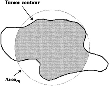
Com=Area∩AreaeqArea, Com
=
Area
∩
Area
eq
Area
,
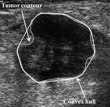
Sol=AreaConvex_area, Sol
=
Area
Convex_area
,
and
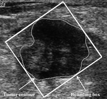
Rec=AreaAreabb, Rec
=
Area
Area
bb
,
where P is the perimeter of the tumor, measured by counting the number of pixels on the tumor margin. In Figure 1 , Area eq is a circle centered at the tumor’s centroid, with an equivalent size as Area. Additionally, Convex_area is the proportion of the pixels in the convex hull, as shown in Figure 2 . The minimum bounding box, Area bb , is a rectangle completely containing the region of tumor, as shown in Figure 3 .
Get Radiology Tree app to read full this article<
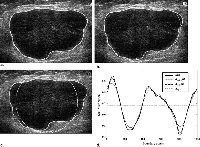
Original NRL Features
Get Radiology Tree app to read full this article<
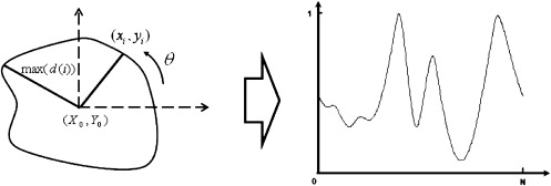
d(i)=[x(i)−X0]2+[y(i)−Y0]2√max[d(i)],i=1,2,…,N, d
(
i
)
=
[
x
(
i
)
−
X
0
]
2
+
[
y
(
i
)
−
Y
0
]
2
max
[
d
(
i
)
]
,
i
=
1
,
2
,
…
,
N
,
where ( x i , y i ) represents each pixel on the tumor contour, ( X 0 , Y 0 ) represents the pixels at the centroid of the tumor image, N is the total number of the pixels on the tumor contour, and max[ d ( i )] is the maximum value of d ( i ).
Get Radiology Tree app to read full this article<
Get Radiology Tree app to read full this article<
New NRL Features
Get Radiology Tree app to read full this article<
Get Radiology Tree app to read full this article<
Difference of Standard Deviation (σ diff )
Get Radiology Tree app to read full this article<
σdiff=|σ−σma| σ
diff
=
|
σ
−
σ
ma
|
where σ is the standard deviation of d ( i ), σ ma is the standard deviation of d ma ( i ), and d ma ( i ) is the result of d ( i ) filtered using the moving-average filter.
Get Radiology Tree app to read full this article<
Get Radiology Tree app to read full this article<
Entropy of the Difference Between d(i) and d ma (i) (Entropy diff )
Get Radiology Tree app to read full this article<
Entropydiff=−∑100k=1pklog(pk), Entropy
diff
=
−
∑
k
=
1
100
p
k
log
(
p
k
)
,
where p k is the probability of | d ( i ) − d ma ( i )|, which was divided into 100 equal parts in the range of [0,1]. Entropy diff is similar to Entropy; d ( i ) is replaced with | d ( i ) − d ma ( i )|. Entropy diff was the measurement of the distribution for the difference between d ( i ) and d ma ( i ). As the NRL approaches regularity, its Entropy diff value will decrease.
Get Radiology Tree app to read full this article<
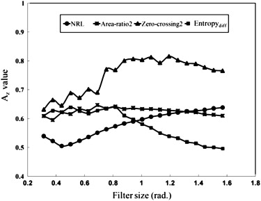
Area Ratio of the Protuberance Outside d ma (i) to the Average Area, N·d avg (Area-ratio2)
Get Radiology Tree app to read full this article<
Area-ratio2=1N⋅davg∑Ni=1[d(i)−dma(i)], Area-ratio2
=
1
N
⋅
d
avg
∑
i
=
1
N
[
d
(
i
)
−
d
ma
(
i
)
]
,
where d ( i ) − d ma ( i ) = 0, ∀d(i)≤dma(i) ∀
d
(
i
)
≤
d
ma
(
i
) . Area-ratio2 represents the area of the lobulated contour in the tumor and was used to measure the protuberance. The moving-average filter size applied in Area-ratio2 was tested by searching for an appropriate value ( Fig 6 ).
Get Radiology Tree app to read full this article<
Zero-crossing Count (Zero-crossing2)
Get Radiology Tree app to read full this article<
Turning Points of NRL (Turning-point)
Get Radiology Tree app to read full this article<
Data Analysis
Classification
Get Radiology Tree app to read full this article<
Radiologists’ Rankings
Get Radiology Tree app to read full this article<
Result Comparison
Get Radiology Tree app to read full this article<
Get Radiology Tree app to read full this article<
Results
Get Radiology Tree app to read full this article<
Table 1
Database of Different Histologic Subtypes, with Corresponding Diameters and Numbers of Soft Tissue Tumors
Benign Tumor Diameter (cm) Number Malignant Tumor Diameter (cm) Number Lipoma 2.6–9.1 19 Metastasis 8.1–11.1 9 Giant cell 2.6–7 9 Malignant Fibrous histiocytoma 8.8–10.9 7 Glomus 1.3–2.8 8 Liposarcoma 8.4–14.3 6 Cavernous hemangioma 1.2–6.6 7 Lymphoma 6.3–12 4 Schwannoma 3.7–6.4 7 Alveolar soft part sarcoma 7.6–8.2 3 Fibroma 3.3–5.6 5 Epithelioid sarcoma 4.9–13.3 3 Neurofibroma 3.3–8.5 5 Hemangiopericytoma 4.2–5.7 2 Aneurysm 4.6–8.9 4 Fibromyxoid sarcoma 8.2 1 Vascular leiomyoma 3.5–4.7 4 Synovial sarcoma 11 1 Benign fibrous histiocytoma 2.6 1 Dermatofibrosarcoma 7 1 Glomangioma 4 1 Total 70 37
Get Radiology Tree app to read full this article<
Get Radiology Tree app to read full this article<
Get Radiology Tree app to read full this article<
Table 2
Individual Performance of the 16 Features Represented by A z and Student’s t Test
Class Feature_A z__P_ Geometric features Area 0.79 ± 0.04 <.001 Circularity 0.60 ± 0.06 .053 Solidity 0.85 ± 0.04 <.001 Compactness 0.78 ± 0.04 <.001 Rectangularity 0.73 ± 0.05 <.001 Old NRL features_d_ avg 0.51 ± 0.06 .484 Σ 0.59 ± 0.06 .089 Entropy 0.53 ± 0.06 .879 Area-ratio1 0.57 ± 0.06 .233 Roughness 0.77 ± 0.05 <.001 Zero-crossing1 0.61 ± 0.06 <.05 New NRL features σ diff ∗ 0.63 ± 0.06 <.05 Entropy diff ∗ 0.64 ± 0.06 <.05 Area-ratio2 ∗ 0.64 ± 0.06 <.05 Zero-crossing2 ∗ 0.81 ± 0.05 <.001 Turning-point 0.66 ± 0.06 <.05
A z , area under the receiver-operating characteristic curve; NRL, normalized radial length.
∗ The resultant features filtered by the optimal moving-average filter.
Get Radiology Tree app to read full this article<
Get Radiology Tree app to read full this article<
Table 3
Linear Discriminant Analysis Performance of Optimal Subsets of the Original NRL and New NRL Features
Class Feature Subset Accuracy Sensitivity Specificity_A z_ Old NRL Roughness, Zero-crossing1 80.4% 64.9% 88.6% 0.79 ± 0.05 New NRL Zero-crossing2, Entropy diff 85.0% 73.0% 91.4% 0.85 ± 0.05
A z , area under the receiver-operating characteristic curve; NRL, normalized radial length.
Get Radiology Tree app to read full this article<
Get Radiology Tree app to read full this article<
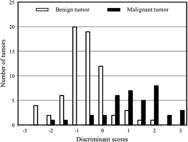
y=4.39×Zero-crossing2+0.25×Entropydiff−45.7×Cir−48.72×σdiff−3.47×Rec−2.72, y
=
4.39
×
Zero-crossing
2
+
0.25
×
Entropy
diff
−
45.7
×
Cir
−
48.72
×
σ
diff
−
3.47
×
Rec
−
2.72
,
where the output value y was used as the discriminant score. Our proposed CAD method was based on this discriminant function, which classifies an STT as benign if y < 0 and malignant if y ≥ 0. The discriminant scores were calculated on the basis of the five feature subsets, as shown in Figure 8 . This distribution represents the classification results for each tumor.
Table 4
Linear Discriminant Analysis Performance of the Optimal Feature Subset, Including the Five Features
Feature Subset Accuracy Sensitivity Specificity PPV NPV_A z_ Zero-crossing2, Entropy diff , circularity, σ diff , rectangularity 87.9% 89.2% 87.1% 78.6% 93.8% 0.93 ± 0.03
A z , area under the receiver-operating characteristic curve; NPV, negative predictive value; PPV, positive predictive value.
Get Radiology Tree app to read full this article<
Get Radiology Tree app to read full this article<
Table 5
Correlations Between Pathologic Results and Radiologists’ Rankings and Between Pathologic Results and CAD Results
Category Correlation_P_ Pathologic results vs radiologist A 0.62 <.01 Pathologic results vs radiologist B 0.61 <.01 Pathologic results vs CAD results 0.73 <.01
CAD, computer-aided diagnosis.
Get Radiology Tree app to read full this article<
Discussion
Get Radiology Tree app to read full this article<
Get Radiology Tree app to read full this article<
Get Radiology Tree app to read full this article<
Get Radiology Tree app to read full this article<
Get Radiology Tree app to read full this article<
Get Radiology Tree app to read full this article<
Get Radiology Tree app to read full this article<
References
1. Jemal A., Tiwari R.C., Murray T., et. al.: Cancer statistics, 2004. CA Cancer J Clin 2004; 54: pp. 8-29.
2. Olsson H.: An updated review of the epidemiology of soft tissue sarcoma. Acta Orthop Scand Suppl 2004; 75: pp. 16-20.
3. Chiou H.J., Chou Y.H., Chiou S.Y., et. al.: Superficial soft-tissue lymphoma: sonographic appearance and early survival. Ultrasound Med Biol 2006; 32: pp. 1287-1297.
4. Chiou H.J., Chou Y.H., Chiou S.Y., Wang H.K.: High-resolution ultrasonography in superficial soft tissue tumors. J Med Ultrasound 2007; 15: pp. 152-174.
5. García-Gómez J.M., Vidal C., Martí-Bonmatí L., et. al.: Benign/malignant classifier of soft tissue tumors using MR imaging. MAGMA 2004; 16: pp. 194-201.
6. Kransdorf M.J., Murphey M.D.: Radiologic evaluation of soft-tissue masses: a current perspective. AJR Am J Roentgenol 2000; 175: pp. 575-587.
7. Verstraete K.L., Vanzieleghem B., De Deene Y., et. al.: Static, dynamic and first-pass MR imaging of musculoskeletal lesions using gadodiamide injection. Acta Radiol 1995; 36: pp. 27-36.
8. Clark M.A., Fisher C., Judson I., Thomas J.M.: Soft-tissue sarcomas in adults. N Engl J Med 2005; 353: pp. 701-711.
9. Gandhi M.R., Benson M.D.: Ultrasound of soft tissue masses. World J Surg 2000; 24: pp. 227-231.
10. Stavros A.T., Thickman D., Rapp C.L., Dennis M.A., Parker S.H., Sisney G.A.: Solid breast nodules: use of sonography to distinguish between benign and malignant lesions. Radiology 1995; 196: pp. 123-134.
11. De Schepper A.M., De Beuckeleer L., Vandevenne J., Somville J.: Magnetic resonance imaging of soft tissue tumors. Eur Radiol 2000; 10: pp. 213-223.
12. Skaane P., Engedal K.: Analysis of sonographic features in the differentiation of fibroadenoma and invasive ductal carcinoma. AJR Am J Roentgenol 1998; 170: pp. 109-114.
13. Kilday J., Palmieri F., Fox M.D.: Classifying mammographic lesions using computerized image analysis. IEEE Trans Med Imaging 1993; 12: pp. 664-669.
14. Chou Y.H., Tiu C.M., Hung G.S., Wu S.C., Chang T.Y., Chiang H.K.: Stepwise logistic regression analysis of tumor contour features for breast ultrasound diagnosis. Ultrasound Med Biol 2001; 27: pp. 1493-1498.
15. Chen C.M., Chou Y.H., Han K.C., et. al.: Breast lesions on sonograms: computer-aided diagnosis with nearly setting-independent features and artificial neural networks. Radiology 2003; 226: pp. 504-514.
16. Chang R.F., Wu W.J., Moon W.K., Chen D.R.: Automatic ultrasound segmentation and morphology based diagnosis of solid breast tumors. Breast Cancer Res Treat 2005; 89: pp. 179-185.
17. Sintzoff S.J., Gillard I., Van G.D., Gevenois P., Salmon I., Struyven J.: Ultrasound evaluation of soft tissue tumors. J Belge Radiol 1992; 75: pp. 276-280.
18. Petrick N., Chan H.P., Wei D., Sahiner B., Helvie M.A., Adler D.D.: Automated detection of breast masses on mammograms using adaptive contrast enhancement and texture classification. Med Phys 1996; 23: pp. 1685-1696.
19. Fisher R.: The use of multiple measurements in taxonomic problems. Ann Eugenics 1936; 7: pp. 179-188.
20. Huang Y.L., Chen D.R., Jiang Y.R., Kuo S.J., Wu H.K., Moon W.K.: Computer-aided diagnosis using morphological features for classifying breast lesions on ultrasound. Ultrasound Obstet Gynecol 2008; 32: pp. 565-572.
21. Kim K.G., Cho S.W., Min S.J., Kim J.H., Min B.G., Bae K.T.: Computerized scheme for assessing ultrasonograpohic features of breast masses. Acad Radiol 2005; 12: pp. 58-66.
22. Alvarenga A.V., Pereira W.C., Infantosi A.F., Azevedo C.M.: Complexity curve and grey level co-occurrence matrix in the texture evaluation of breast tumor on ultrasound images. Med Phys 2007; 34: pp. 379-387.
23. Wu W.J., Moon W.K.: Ultrasound breast tumor image computer-aided diagnosis with texture and morphological features. Acad Radiol 2008; 15: pp. 873-880.