CT-based Radiomics Signature to Discriminate High-grade From Low-grade Colorectal Adenocarcinoma

Rationale and Objectives

To develop and validate a computed tomography-based radiomics signature for preoperatively discriminating high-grade from low-grade colorectal adenocarcinoma (CRAC).

Materials and Methods

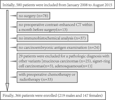
This retrospective study was approved by our institutional review board, and the informed consent requirement was waived. This study enrolled 366 patients with CRAC (training dataset: n = 222, validation dataset: n = 144) from January 2008 to August 2015. A radiomics signature was developed with the least absolute shrinkage and selection operator method in training dataset. Mann-Whitney U test was applied to explore the correlation between radiomics signature and histologic grade. The discriminative power of radiomics signature was investigated with the receiver operating characteristics curve. An independent validation dataset was used to confirm the predictive performance. We further performed a stratified analysis to validate the predictive performance of radiomics signature in colon adenocarcinoma and rectal adenocarcinoma.

Results

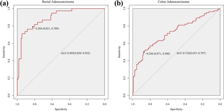
The radiomics signature demonstrated discriminative performance for high-grade and low-grade CRAC, with an area under the curve of 0.812 (95% confidence interval [CI]: 0.749–0.874) in training dataset and 0.735 (95%CI: 0.644–0.826) in validation dataset. Stratified analysis demonstrated that radiomics signature also showed distinguishing ability for histologic grade in both colon adenocarcinoma and rectal adenocarcinoma, with area under the curve of 0.725 (95%CI: 0.653–0.797) and 0.895 (95%CI: 0.838–0.952), respectively.

Conclusions

We developed and validated a radiomics signature as a complementary tool to differentiate high-grade from low-grade CRAC preoperatively, which may make contribution to personalized treatment.

Introduction

Colorectal cancer (CRC) is one of the most common cancers globally, ranking the third and fourth as a cause of cancer-related death in women and men, respectively . Colorectal adenocarcinoma (CRAC) is the most common histologic type, accounting for more than 90% of CRC . The degree of differentiation of CRAC was demonstrated by numerous studies as a significant factor for prognosis . A two-tiered classification system of histologic grade (low grade = well and moderate differentiation; high grade = poor differentiation) was recommended in CRAC for better reproducibility and prognostic significance . Specifically, high-grade CRAC had higher risk to relapse after tumor resection, resulting in poorer prognosis . Preoperatively, radiotherapy or chemoradiotherapy could improve local control and disease-free survival in high-risk patients with rectal cancers . However, neoadjuvant therapies also have been reported for serious side effects, such as occurrence of second cancers and adverse effects on anorectal function . Thus, to achieve maximum benefit and avoid unnecessary side effects caused by preoperatively excessive treatment, discriminating high-grade from low-grade CRAC to assist in identifying patients with high risk of recurrence before treatment would be vital for individual therapy and hence improving outcomes.

To preoperatively evaluate histologic grade, pathologic assessment of biopsy samples could offer some information of tumor differentiation, because colonoscopic biopsy is regularly used to diagnose CRC . However, as tumors were heterogeneous in space , the discrepancy may occur between biopsy and surgical specimen for evaluating histologic grade, because biopsy samples may be superficial, inadequate, or poorly oriented . Additionally, colonoscopic biopsy as an invasive examination has related side effects .

Get Radiology Tree app to read full this article<

Materials and Methods

Patients

Get Radiology Tree app to read full this article<

Assessment of Histologic Grade

Get Radiology Tree app to read full this article<

Acquisition of CT Image

Get Radiology Tree app to read full this article<

Radiomics Feature Extraction

Get Radiology Tree app to read full this article<

Statistical Analysis

Get Radiology Tree app to read full this article<

Radiomics Feature Selection and Radiomics Signature Building

Get Radiology Tree app to read full this article<

Predictive Performance of Radiomics Signature

Get Radiology Tree app to read full this article<

Stratified Analysis for Radiomics Signature in Colon and Rectal Adenocarcinoma

Get Radiology Tree app to read full this article<

Results

Clinical Characteristics

Get Radiology Tree app to read full this article<

TABLE 1

Characteristics of Patients in the Training and Validation Datasets

Training Dataset Validation Dataset Characteristics Low Grade High Grade_P_ † Low Grade High Grade_P_ † Age, mean ± SD, y 61.26 ± 13.33 59.55 ± 13.19 .369 60.35 ± 11.82 63.54 ± 12.01 .132 Gender, No. (%) Male 91 (61.5) 44 (59.5) .771 55 (57.3) 29 (60.4) .720 Female 57 (38.5) 30 (40.5) 41 (42.7) 19 (39.6) CT-reported tumor location Right-sided colon 24 (16.2) 29 (38.2) <.001 12 (12.5) 18 (37.5) <.001 Others \* 124 (83.8) 45 (61.8) 84 (87.5) 30 (62.5) CEA level, No. (%) Normal 85 (57.4) 46 (62.2) .499 61 (63.5) 30 (62.5) .903 Abnormal 63 (42.6) 28 (37.8) 35 (36.5) 18 (37.5) Radiomics score median (interquartile range) −1.548 (−2.348 to −0.680) 0.333 (−0.811 to 1.008) <.001 −1.594 (−2.432 to −0.881) −0.118 (−1.476 to 1.086) <.001

Abbreviations: CEA, carcinoembryonic antigen; CT, computed tomography; SD, standard deviation; No. (%), the numbers before parentheses represent the actual numbers and the numbers within parentheses represent corresponding percentages.

Get Radiology Tree app to read full this article<

Statistical Analysis of Pathologic Findings of Biopsy

Get Radiology Tree app to read full this article<

TABLE 2

The Pathologic Findings of Colonoscopic Biopsy

Training Dataset Validation Dataset Pathologic Findings of Biopsy, No. (%) Low Grade High Grade Low Grade High Grade Low-grade CRAC 67 (45.3) 22 (29.7) 43 (44.8) 11 (22.9) High-grade CRAC 1 (0.7) 13 (17.6) 1 (1.0) 19 (39.6) CRAC without grade \* 56 (37.8) 21 (28.4) 40 (41.7) 14 (29.2) Non-cancer † 5 (3.4) 2 (2.7) 1 (1.0) 2 (4.2) Without a biopsy 19 (12.8) 16 (21.6) 11 (11.5) 2 (4.2)

Abbreviations: CRAC, colorectal adenocarcinoma; No. (%), the numbers before parentheses represent the actual numbers and the numbers within parentheses represent corresponding percentages.

Get Radiology Tree app to read full this article<

Reproducibility of Radiomics Feature Extraction

Get Radiology Tree app to read full this article<

Radiomics Feature Selection and Radiomics Signature Building

Get Radiology Tree app to read full this article<

Predictive Performance of Radiomics Signature

Get Radiology Tree app to read full this article<

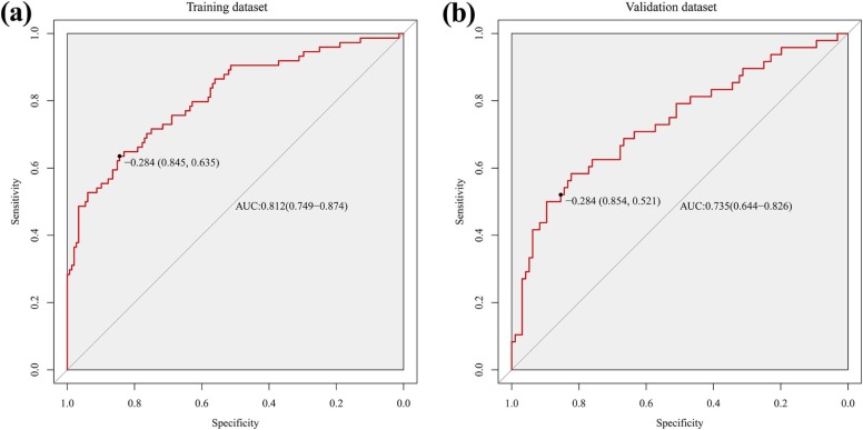
TABLE 3

Predictive Performance of Radiomics Signature

Predictive Performance AUC (95%CI) SEN SPE PPV NPV Accuracy Training dataset 0.812 (0.749–0.874) 0.635 0.845 0.671 0.822 0.775 Validation dataset 0.735 (0.644–0.826) 0.521 0.854 0.641 0.781 0.743 Rectal adenocarcinoma 0.895 (0.838–0.952) 0.789 0.821 0.600 0.920 0.813 Colon adenocarcinoma 0.725 (0.653–0.797) 0.500 0.871 0.712 0.732 0.727

Abbreviations: AUC, area under curve; CI, confidence interval; SEN, sensitivity; SPE, specificity; PPV, positive predictive value; NPV, negative predictive value.

Get Radiology Tree app to read full this article<

Stratified Analysis for Radiomics Signature in Colon and Rectal Adenocarcinoma

Get Radiology Tree app to read full this article<

Discussion

Get Radiology Tree app to read full this article<

Conclusion

Get Radiology Tree app to read full this article<

Acknowledgments

Get Radiology Tree app to read full this article<

Appendix

Appendix A.1

Radiomics Feature Extraction Methodology

Get Radiology Tree app to read full this article<

1. Get Radiology Tree app to read full this article<

Get Radiology Tree app to read full this article<

Energy=∑Ni=1X(i)2 Energy

∑

(

)

Get Radiology Tree app to read full this article<

Kurtosis=1N∑Ni=1(X(i)−X¯¯¯)4(1N∑Ni=1(X(i)−X¯¯¯)2)2 Kurtosis

∑

(

)

−

)

(

∑

(

)

−

)

Get Radiology Tree app to read full this article<

Skewness=1N∑Ni=1(X(i)−X¯¯¯)31N∑Ni=1(X(i)−X¯¯¯)2√3 Skewness

∑

(

)

−

)

∑

(

)

−

)

Get Radiology Tree app to read full this article<

Mean=1N∑Ni=1X(i) Mean

∑

(

)

Get Radiology Tree app to read full this article<

MAD=∑Ni=1∣∣X(i)−X¯¯¯∣∣N MAD

∑

(

)

−

Get Radiology Tree app to read full this article<

RMS=∑Ni=1X(i)2N−−−−−−−√ RMS

∑

(

)

Get Radiology Tree app to read full this article<

SD=1N−1∑Ni=1(X(i)−X¯¯¯)2−−−−−−−−−−−−−−−−−−−√ SD

−

∑

(

)

−

)

Get Radiology Tree app to read full this article<

Variance=1N−1∑Ni=1(X(i)−X¯¯¯)2 Variance

−

∑

(

)

−

)

Get Radiology Tree app to read full this article<

Entropy=−∑N1i=1P(i)log2P(i) Entropy

−

∑

(

)

log

(

)

Get Radiology Tree app to read full this article<

Uniformity=∑N1i=1P(i)2 Uniformity

∑

(

)

Get Radiology Tree app to read full this article<

2. Get Radiology Tree app to read full this article<

Get Radiology Tree app to read full this article<

Compactness1=Vπ√A23 Compactness

Get Radiology Tree app to read full this article<

Compactness2=36πV2A3 Compactness

Get Radiology Tree app to read full this article<

sph_dis=A4πR2 sph_dis

Get Radiology Tree app to read full this article<

Sphericity=π13(6V)23A Sphericity

(

)

Get Radiology Tree app to read full this article<

svr=AV svr

3. Get Radiology Tree app to read full this article<

Get Radiology Tree app to read full this article<

(1) Get Radiology Tree app to read full this article<

Get Radiology Tree app to read full this article<

Get Radiology Tree app to read full this article<

Autocorrelation=∑Ngi=1∑Ngj=1ijP(i,j) Autocorrelation

∑

(

)

Get Radiology Tree app to read full this article<

Clu_pro=∑Ngi=1∑Ngj=1[i+j−μx(i)−μy(j)]4P(i,j) Clu_pro

∑

[

−

(

)

−

(

)

]

(

)

Get Radiology Tree app to read full this article<

Clu_shade=∑Ngi=1∑Ngj=1[i+j−μx(i)−μy(j)]3P(i,j) Clu_shade

∑

[

−

(

)

−

(

)

]

(

)

Get Radiology Tree app to read full this article<

Clu_ten=∑Ngi=1∑Ngj=1[i+j−μx(i)−μy(j)]2P(i,j) Clu_ten

∑

[

−

(

)

−

(

)

]

(

)

Get Radiology Tree app to read full this article<

Get Radiology Tree app to read full this article<

Correlation=∑Ngi=1∑Ngj=1ijP(i,j)−μi(i)μj(j)σx(i)σy(j) Correlation

∑

(

)

−

(

)

(

)

(

)

(

)

Get Radiology Tree app to read full this article<

Diff_entropy=∑Ng−1i=0Px−y(i)log2[Px−y(i)] Diff_entropy

∑

−

(

)

log

[

−

(

)

]

Get Radiology Tree app to read full this article<

Dissimilarity=∑Ngi=1∑Ngj=1|i−j|P(i,j) Dissimilarity

∑

−

(

)

Get Radiology Tree app to read full this article<

Energy=∑Ngi=1∑Ngj=1[P(i,j)]2 Energy

∑

[

(

)

]

Get Radiology Tree app to read full this article<

Entropy=−∑Ngi=1∑Ngj=1P(i,j)log2[P(i,j)] Entropy

−

∑

(

)

log

[

(

)

]

Get Radiology Tree app to read full this article<

Get Radiology Tree app to read full this article<

Homogeneity2=∑Ngi=1∑Ngj=1P(i,j)1+|i−j|2 Homogeneity

∑

(

)

−

Get Radiology Tree app to read full this article<

IMC1=HXY−HXY1max{HX,HY} IMC

−

{

}

Get Radiology Tree app to read full this article<

IMC2=1−e−2|HXY2−HXY|−−−−−−−−−−−−−−−√ IMC

−

Get Radiology Tree app to read full this article<

IDMN=∑Ngi=1∑Ngj=1P(i,j)1+|i−j|2Ng2 IDMN

∑

(

)

−

Get Radiology Tree app to read full this article<

IDN=∑Ngi=1∑Ngj=1P(i,j)1+|i−j|2Ng IDN

∑

(

)

−

Get Radiology Tree app to read full this article<

inv_var=∑Ngi=1∑Ngj=1P(i,j)|i−j|2,(i≠j) inv_var

∑

(

)

−

(

≠

)

sum_average=∑2Ngi=2[iPx+y(i)] sum_average

∑

[

(

)

]

Get Radiology Tree app to read full this article<

sum_entropy=−∑2Ngi=2Px+y(i)log2[Px+y(i)] sum_entropy

−

∑

(

)

log

[

(

)

]

Get Radiology Tree app to read full this article<

sum_var=∑2Ngi=2(i−SE)2Px+y(i) sum_var

∑

(

−

)

(

)

Get Radiology Tree app to read full this article<

variance=∑Ngi=1∑Ngj=1(i−μ)2P(i,j) variance

∑

(

−

)

(

)

(2) Get Radiology Tree app to read full this article<

Get Radiology Tree app to read full this article<

Get Radiology Tree app to read full this article<

SRE=∑Ngi=1∑Nrj=1[p(i,j|θ)j2]∑Ngi=1∑Nrj=1[p(i,j|θ)] SRE

∑

[

(

)

]

∑

[

(

)

]

Get Radiology Tree app to read full this article<

LRE=∑Ngi=1∑Nrj=1j2p(i,j|θ)∑Ngi=1∑Nrj=1[p(i,j|θ)] LRE

∑

(

)

∑

[

(

)

]

Get Radiology Tree app to read full this article<

GLN=∑Ngi=1[∑Nrj=1p(i,j|θ)]2∑Ngi=1∑Nrj=1[p(i,j|θ)] GLN

∑

[

∑

(

)

]

∑

[

(

)

]

Get Radiology Tree app to read full this article<

RLN=∑Nrj=1[∑Ngi=1p(i,j|θ)]2∑Ngi=1∑Nrj=1[p(i,j|θ)] RLN

∑

[

∑

(

)

]

∑

[

(

)

]

Get Radiology Tree app to read full this article<

RP=∑Ngi=1∑Nrj=1p(i,j|θ)Np RP

∑

(

)

Get Radiology Tree app to read full this article<

LGLRE=∑Ngi=1∑Nrj=1[p(i,j|θ)i2]∑Ngi=1∑Nrj=1[p(i,j|θ)] LGLRE

∑

[

(

)

]

∑

[

(

)

]

Get Radiology Tree app to read full this article<

HGLRE=∑Ngi=1∑Nrj=1i2p(i,j|θ)∑Ngi=1∑Nrj=1[p(i,j|θ)] HGLRE

∑

(

)

∑

[

(

)

]

Get Radiology Tree app to read full this article<

SRLGLE=∑Ngi=1∑Nrj=1[p(i,j|θ)i2j2]∑Ngi=1∑Nrj=1[p(i,j|θ)] SRLGLE

∑

[

(

)

]

∑

[

(

)

]

Get Radiology Tree app to read full this article<

SRHGLE=∑Ngi=1∑Nrj=1[p(i,j|θ)i2j2]∑Ngi=1∑Nrj=1[p(i,j|θ)] SRHGLE

∑

[

(

)

]

∑

[

(

)

]

Get Radiology Tree app to read full this article<

LRLGLE=∑Ngi=1∑Nrj=1[p(i,j|θ)j2i2]∑Ngi=1∑Nrj=1[p(i,j|θ)] LRLGLE

∑

[

(

)

]

∑

[

(

)

]

Get Radiology Tree app to read full this article<

LRHGLE=∑Ngi=1∑Nrj=1p(i,j|θ)i2j2∑Ngi=1∑Nrj=1[p(i,j|θ)] LRHGLE

∑

(

)

∑

[

(

)

]

4. Get Radiology Tree app to read full this article<

Get Radiology Tree app to read full this article<

TABLE A.1

Representing Number of Functions on X, Y, Z Scale

Functions on X, Y, Z scale LLL LLH LHL LHH HLL HLH HHL HHH Representing number 1 2 3 4 5 6 7 8

Get Radiology Tree app to read full this article<

Appendix A.2

Statistical Analysis

Appendix A2a

Demographic comparison between patients with low-grade and high-grade CRAC and between training and validation datasets

Get Radiology Tree app to read full this article<

Appendix A2b

The packages of R software used for statistical analysis

Get Radiology Tree app to read full this article<

Appendix A.3

Feature Normalization

Get Radiology Tree app to read full this article<

X′=X−X¯¯¯SD X

′

−

where X is the value of each selected feature in a patient, whereas X′ X

′ is the corresponding normalized value. X¯¯¯ X

¯ represents the mean of the values of the feature, and SD is standard deviation in training dataset. The mean and standard deviation of each features are shown in Table A.2 .

TABLE A.2

Data of z-Score Normalization

Features Mean Standard Deviation db3_4_RMS 1996.043 590.3509 db10_4_RMS 1966.537 577.5884 db10_8_range 469.7477 107.6682 bior3.7_3_energy 9933893 5400296 bior4.4_8_sd 42.64378 11.39670 bior5.5_3_sd 60.44354 17.05864 bior5.5_4_RMS 1990.187 589.9640 bior5.5_5_sd 287.2846 58.48172 dmey_2_sd 63.40118 16.19524 dmey_3_energy 9575864 5159117 dmey_4_sd 44.33686 11.35308 rbio2.2_1_inv_var 0.3163109 0.06468699 rbio2.8_4_sd 49.22477 12.79117 rbio3.9_3_energy 9820202 5332593

Get Radiology Tree app to read full this article<

Appendix A.4

Rad-Score Calculation Formula

Get Radiology Tree app to read full this article<

References

1. Torre L.A., Bray F., Siegel R.L., et. al.: Global cancer statistics, 2012. CA Cancer J Clin 2015; 65: pp. 87-108.
2. Fleming M., Ravula S., Tatishchev S.F., et. al.: Colorectal carcinoma: pathologic aspects. J Gastrointest Oncol 2012; 3: pp. 153-173.
3. Chung C.K., Zaino R.J., Stryker J.A.: Colorectal carcinoma: evaluation of histologic grade and factors influencing prognosis. J Surg Oncol 1982; 21: pp. 143-148.
4. Compton C.C.: Colorectal carcinoma: diagnostic, prognostic, and molecular features. Mod Pathol 2003; 16: pp. 376-388.
5. Derwinger K., Kodeda K., Bexe-Lindskog E., et. al.: Tumour differentiation grade is associated with TNM staging and the risk of node metastasis in colorectal cancer. Acta Oncol 2010; 49: pp. 57-62.
6. Vasile L., Olaru A., Munteanu M., et. al.: Prognosis of colorectal cancer: clinical, pathological and therapeutic correlation. Rom J Morphol Embryol 2012; 53: pp. 383-391.
7. Compton C.C., Fielding L.P., Burgart L.J., et. al.: Prognostic factors in colorectal cancer. College of American Pathologists Consensus Statement 1999. Arch Pathol Lab Med 2000; 124: pp. 979-994.
8. Bosman F.T., World Health Organization, International Agency for Research on Cancer: WHO classification of tumours of the digestive system.2010.IARC PressLyon
9. Onate-Ocana L.F., Montesdeoca R., Lopez-Graniel C.M., et. al.: Identification of patients with high-risk lymph node-negative colorectal cancer and potential benefit from adjuvant chemotherapy. Jpn J Clin Oncol 2004; 34: pp. 323-328.
10. Bockelman C., Engelmann B.E., Kaprio T., et. al.: Risk of recurrence in patients with colon cancer stage II and III: a systematic review and meta-analysis of recent literature. Acta Oncol 2015; 54: pp. 5-16.
11. Sauer R., Becker H., Hohenberger W., et. al.: Preoperative versus postoperative chemoradiotherapy for rectal cancer. N Engl J Med 2004; 351: pp. 1731-1740.
12. Sebag-Montefiore D., Stephens R.J., Steele R., et. al.: Preoperative radiotherapy versus selective postoperative chemoradiotherapy in patients with rectal cancer (MRC CR07 and NCIC-CTG C016): a multicentre, randomised trial. Lancet 2009; 373: pp. 811-820.
13. Birgisson H., Pahlman L., Gunnarsson U., et. al.: Occurrence of second cancers in patients treated with radiotherapy for rectal cancer. J Clin Oncol 2005; 23: pp. 6126-6131.
14. Canda A.E., Terzi C., Gorken I.B., et. al.: Effects of preoperative chemoradiotherapy on anal sphincter functions and quality of life in rectal cancer patients. Int J Colorectal Dis 2010; 25: pp. 197-204.
15. Brenner H., Kloor M., Pox C.P.: Colorectal cancer. Lancet 2014; 383: pp. 1490-1502.
16. Gerlinger M., Rowan A.J., Horswell S., et. al.: Intratumor heterogeneity and branched evolution revealed by multiregion sequencing. N Engl J Med 2012; 366: pp. 883-892.
17. Aerts H.J., Velazquez E.R., Leijenaar R.T., et. al.: Decoding tumour phenotype by noninvasive imaging using a quantitative radiomics approach. Nat Commun 2014; 5: pp. 4006.
18. Kim J.E., Lee J.M., Baek J.H., et. al.: Differentiation of poorly differentiated colorectal adenocarcinomas from well- or moderately differentiated colorectal adenocarcinomas at contrast-enhanced multidetector CT. Abdom Imaging 2015; 40: pp. 1-10.
19. Viiala C.H., Zimmerman M., Cullen D.J., et. al.: Complication rates of colonoscopy in an Australian teaching hospital environment. Intern Med J 2003; 33: pp. 355-359.
20. Senore C., Ederle A., Fantin A., et. al.: Acceptability and side-effects of colonoscopy and sigmoidoscopy in a screening setting. J Med Screen 2011; 18: pp. 128-134.
21. Leufkens A.M., van den Bosch M.A., van Leeuwen M.S., et. al.: Diagnostic accuracy of computed tomography for colon cancer staging: a systematic review. Scand J Gastroenterol 2011; 46: pp. 887-894.
22. Kumar V., Gu Y., Basu S., et. al.: Radiomics: the process and the challenges. Magn Reson Imaging 2012; 30: pp. 1234-1248.
23. Lambin P., Rios-Velazquez E., Leijenaar R., et. al.: Radiomics: extracting more information from medical images using advanced feature analysis. Eur J Cancer 2012; 48: pp. 441-446.
24. Gillies R.J., Kinahan P.E., Hricak H.: Radiomics: images are more than pictures, they are data. Radiology 2016; 278: pp. 563-577.
25. Huang Y., Liu Z., He L., et. al.: Radiomics signature: a potential biomarker for the prediction of disease-free survival in early-stage (I or II) non-small cell lung cancer. Radiology 2016; 281: pp. 947-957.
26. Huang Y.Q., Liang C.H., He L., et. al.: Development and validation of a radiomics nomogram for preoperative prediction of lymph node metastasis in colorectal cancer. J Clin Oncol 2016; 34: pp. 2157-2164.
27. Liang C., Huang Y., He L., et. al.: The development and validation of a CT-based radiomics signature for the preoperative discrimination of stage I-II and stage III-IV colorectal cancer. Oncotarget 2016; 7: pp. 31401-31412.
28. Gstoettner M., Sekyra K., Walochnik N., et. al.: Inter- and intraobserver reliability assessment of the Cobb angle: manual versus digital measurement tools. Eur Spine J 2007; 16: pp. 1587-1592.
29. Zhu L., Pan Z., Ma Q., et. al.: Diffusion kurtosis imaging study of rectal adenocarcinoma associated with histopathologic prognostic factors: preliminary findings. Radiology 2017; 284: pp. 66-76.
30. Lubner M.G., Stabo N., Lubner S.J., et. al.: CT textural analysis of hepatic metastatic colorectal cancer: pre-treatment tumor heterogeneity correlates with pathology and clinical outcomes. Abdom Imaging 2015; 40: pp. 2331-2337.
31. Liu F., Li C., Jia H., et. al.: Is there a prognostic value of tumor location among Chinese patients with colorectal cancer?. Oncotarget 2017; 8: pp. 38682-38692.
32. Ueno H., Kajiwara Y., Shimazaki H., et. al.: New criteria for histologic grading of colorectal cancer. Am J Surg Pathol 2012; 36: pp. 193-201.
33. Kinoshita O., Kishimoto M., Murayama Y., et. al.: Poorly differentiated clusters with larger extents have a greater impact on survival: a semi-quantitative pathological evaluation for 239 patients with non-mucinous pT2-3 colorectal carcinoma. World J Surg Oncol 2015; 13: pp. 140.

CT-based Radiomics Signature to Discriminate High-grade From Low-grade Colorectal Adenocarcinoma

Rationale and Objectives

Materials and Methods

Results

Conclusions

Introduction

Materials and Methods

Patients

Assessment of Histologic Grade

Acquisition of CT Image

Radiomics Feature Extraction

Statistical Analysis

Radiomics Feature Selection and Radiomics Signature Building

Predictive Performance of Radiomics Signature

Stratified Analysis for Radiomics Signature in Colon and Rectal Adenocarcinoma

Results

Clinical Characteristics

Statistical Analysis of Pathologic Findings of Biopsy

Reproducibility of Radiomics Feature Extraction

Radiomics Feature Selection and Radiomics Signature Building

Predictive Performance of Radiomics Signature

Stratified Analysis for Radiomics Signature in Colon and Rectal Adenocarcinoma

Discussion

Conclusion

Acknowledgments

Appendix

Appendix A.1

Radiomics Feature Extraction Methodology

Appendix A.2

Statistical Analysis

Appendix A2a

Demographic comparison between patients with low-grade and high-grade CRAC and between training and validation datasets

Appendix A2b

The packages of R software used for statistical analysis

Appendix A.3

Feature Normalization

Appendix A.4

Rad-Score Calculation Formula

References

Further Reading

Advanced Modeled Iterative Reconstruction (ADMIRE) Facilitates Radiation Dose Reduction in Abdominal CT

Building a Tree From the Leaves Down A Challenge for Contemporary Educators

Characterization of Urinary Stone Composition by Use of Whole-body, Photon-counting Detector CT