Differentiation of Lipoma From Liposarcoma on MRI Using Texture and Shape Analysis

Rationale and Objectives

To determine if differentiation of lipoma from liposarcoma on magnetic resonance imaging can be improved using computer-assisted diagnosis (CAD).

Materials and Methods

Forty-four histologically proven lipomatous tumors (24 lipomas and 20 liposarcomas) were studied retrospectively. Studies were performed at 1.5T and included T 1 -weighted, T 2 -weighted, T 2 -fat-suppressed, short inversion time inversion recovery, and contrast-enhanced sequences. Two experienced musculoskeletal radiologists blindly and independently noted their degree of confidence in malignancy using all available images/sequences for each patient. For CAD, tumors were segmented in three dimensions using T 1 -weighted images. Gray-level co-occurrence and run-length matrix textural features, as well as morphological features, were extracted from each tumor volume. Combinations of shape and textural features were used to train multiple, linear discriminant analysis classifiers. We assessed sensitivity, specificity, and accuracy of each classifier for delineating lipoma from liposarcoma using 10-fold cross-validation. Diagnostic accuracy of the two radiologists was determined using contingency tables. Interreader agreement was evaluated by Cohen kappa.

Results

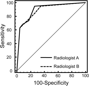
Using optimum-threshold criteria, CAD produced superior values (sensitivity, specificity, and accuracy are 85%, 96%, and 91%, respectively) compared to radiologist A (75%, 83%, and 80%) and radiologist B (80%, 75%, and 77%). Interreader agreement between radiologists was substantial (kappa [95% confidence interval] = 0.69 [0.48–0.90]).

Conclusions

CAD may help radiologists distinguish lipoma from liposarcoma.

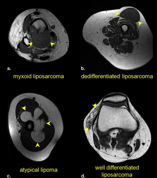
Lipomatous tumors, either benign or malignant, account for approximately half of all soft tissue tumors . Moreover, 16%–18% of malignant soft tissue sarcomas are liposarcomas . Magnetic resonance imaging (MRI) is the standard of care for the imaging workup of lipomatous tumors . Compared to liposarcomas, lipomas are frequently smaller, have more distinct margins, exhibit homogenous T 1 -weighted signal, are completely suppressed on selective fat-suppressed T 1 - and T 2 -weighted sequences as well as short inversion time inversion recovery (STIR) imaging, and show little to no contrast enhancement. On the other hand, liposarcomas are typically larger and more heterogeneous, with a decreased percentage of mature fat composition and contain more nodular or globular areas of nonadipose tissue . Despite these well-known criteria, there is substantial overlap between these conventional radiological criteria , especially in differentiating simple lipomas from atypical lipomas and well-differentiated liposarcomas. In contrast to tertiary cancer centers, most radiologists in general practice see relatively few extremity liposarcomas in their routine practice, rendering the practical application of these rules difficult . When radiologic techniques fail to provide a clear differentiation of these tumors, a biopsy or resection is usually performed. Biopsy may be difficult, especially for abdominal and pelvic tumors, which are often large, deep, and may be difficult to access. When image-guided biopsy is performed on fatty tumors, the biopsy generally targets the most nonadipose component of the lesion. Biopsy, however, can be vulnerable to sampling errors and can potentially facilitate local tumor spread . Therefore, a need exists for a less subjective imaging method that could help distinguish lipoma from liposarcoma.

Computer-assisted diagnosis (CAD) techniques have been applied to help with clinical interpretation of several types of tumors . Some of these CAD techniques have used image features such as texture . We sought to apply a similar algorithm to lipomatous tumors. Thus, we compared experienced musculoskeletal radiologists to CAD in terms of their ability to distinguish lipomas from liposarcomas on magnetic resonance (MR) images.

Materials and methods

Study Population

Get Radiology Tree app to read full this article<

Table 1

Anatomic Locations of Tumors

Location of Lesion Total Number of Lipomatous Lesions Number of Lipomas Number of Liposarcomas Rectus muscle 1 0 1 Scapula 1 1 0 Thigh 16 8 8 Shoulder 12 11 1 Iliopsoas 1 1 0 Elbow 1 0 1 Calf 2 0 2 Popliteal fossa 3 0 3 Arm 3 1 2 Knee 1 0 1 Hand 1 1 0 Chest wall 1 1 0 Tibia and fibula 1 0 1

Get Radiology Tree app to read full this article<

MRI Protocol

Get Radiology Tree app to read full this article<

Subjective Interpretation

Get Radiology Tree app to read full this article<

Computer-Aided Diagnosis

Get Radiology Tree app to read full this article<

Statistics

Get Radiology Tree app to read full this article<

Results

Get Radiology Tree app to read full this article<

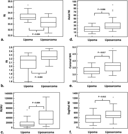
Table 2

Receiver Operating Characteristics of Individual Texture and Shape Features

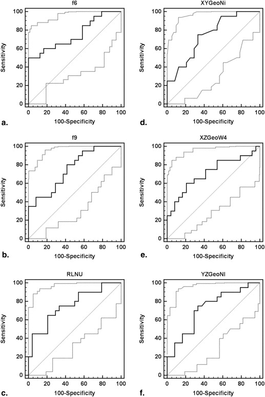
Feature Definition AUC SE_P_ Value Criterion Sensitivity (%) Specificity (%)F6 a ∑2Ngi=2ipx+y(i) ∑

(

) 0.75 0.08 .0010 ≤33.0 50.0 100F9 a −∑Ngi=1∑Ngj=1P(i,j)Rlog(P(i,j)R) −

∑

(

)

log

(

)

) 0.75 0.07 .0005 >2.17 80.0 58.3RLNU b ∑Ngj=1(∑Nri=1p(i,j))2∑Ngi=1∑Nrj=1p(i,j) ∑

(

∑

(

)

∑

(

) 0.76 0.07 .0005 >23,537 65.0 79.2 XY Ni Number of branches on the topological skeleton (axial) 0.74 0.07 .0011 >21 75.0 66.7 XZ W4 Convexity of the shape (coronal)

∑ProfilePerimeterConvexPerimeter ∑

ProfilePerimeter

ConvexPerimeter 0.71 0.08 .0103 >3.52 60.0 79.2 YZ Nl Number of profile contour pixels (sagittal) 0.72 0.08 .0046 >401 75.0 66.7

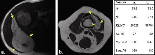
AUC, area under the curve; SE, standard error of the AUC; RLNU, run-length nonuniformity; XY Ni , the number of branches on the topological skeleton in the central XY image; XY W4 , convexity of the tumor in the central XZ image; YZ Nl , perimeter of the tumor contour in the central YZ image.

Get Radiology Tree app to read full this article<

Table 3

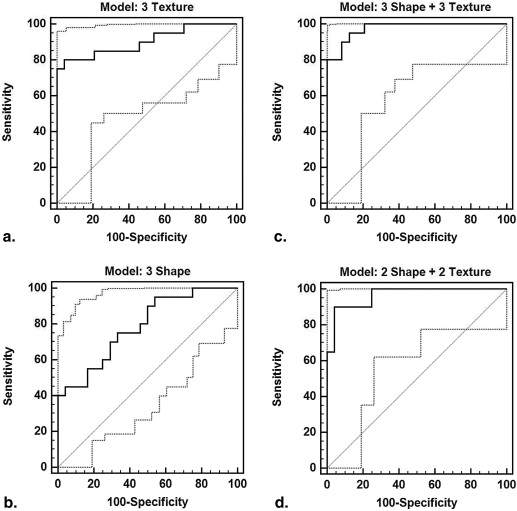
Receiver Operator Characteristics for Feature Combinations

Logistic Regression Model AUC SE (AUC)P Value Criterion Sensitivity (%) Specificity (%) Three shape + three texture 0.98 0.02 <.0001 >0.17 95.0 87.5 Top 4: f6 , f9 , XY Ni , XZ W4 a 0.97 0.02 <.0001 >0.37 90.0 95.8 Texture: f6 , f9 , RLNU b,f 0.90 0.05 <.0001 >0.54 80.0 95.8 Shape: XY Ni , XZ W4 , YZ Nl c,e 0.79 0.07 <.0001 >0.36 75.0 66.7 Texture: f6 , f9 c 0.88 0.05 <.0001 >0.49 75.0 91.7 Shape: XY Ni , XZ W4 d 0.77 0.07 .0001 >0.31 80.0 62.5

a No significant difference in AUC between logistic regression model created with all six features and the model generated with the top four features ( P = .53), b the three texture features ( P = .12), or c the two texture features ( P = .05), although it was superior to the model generated with both c the three shape features ( P = .003) and d the two shape features ( P = .003). e The AUC associated with the model created with the top four features was also significantly greater than that which was generated with the three shape features ( P = .004) but was not superior to the model created with f the three texture features ( P = .18).

Get Radiology Tree app to read full this article<

Table 4

Sensitivity, Specificity, and Accuracy of CAD Feature Combinations After Cross-Validation

LDA Classifier Ten-Fold Cross-Validation Sensitivity Specificity Accuracy Three shape + three texture 88 90 89 Top 4: f6 , f9 , XY Ni , XZ W4 85 96 91 Top 3: f6 , f9 , XY Ni 78 95 87 Texture: f6 , f9 , run-length nonuniformity 78 92 85 Shape: XY Ni , XZ W4 , YZ Nl 78 75 76

CAD, computer-assisted diagnosis; LDA, linear discriminant analysis; XY Ni , the number of branches on the topological skeleton in the central XY image; XY W4 , convexity of the tumor in the central XZ image; YZ Nl , perimeter of the tumor contour in the central YZ image.

Get Radiology Tree app to read full this article<

Table 5

Optimal Results by CAD (Four Features Combined, with Cross-Validation) and Radiologists for Differentiating Lipoma From Liposarcoma

Sensitivity (%) Specificity (%) Accuracy (%) CAD 85 96 91 Radiologist A 75 83 80 Radiologist B 80 75 77

CAD, computer-assisted diagnosis.

Get Radiology Tree app to read full this article<

Discussion

Get Radiology Tree app to read full this article<

Conclusions

Get Radiology Tree app to read full this article<

References

1. Weiss S.W.: Lipomatous tumors. Monogr Pathol 1996; 38: pp. 207-239.
2. Rydholm A., Berg N.O.: Size, site and clinical incidence of lipoma. Factors in the differential diagnosis of lipoma and sarcoma. Acta Orthop Scand 1983; 54: pp. 929-934.
3. Myhre-Jensen O.: A consecutive 7-year series of 1331 benign soft tissue tumors. Clinicopathologic data. Comparison with sarcomas. Acta Orthop Scand 1981; 52: pp. 287-293.
4. Kransdorf M.J., Bancroft L.W., Peterson J.J., et. al.: Imaging of fatty tumors: distinction of lipoma and well-differentiated liposarcoma. Radiology 2002; 224: pp. 99-104.
5. Munk P.L., Lee M.J., Janzen D.L., et. al.: Lipoma and liposarcoma: evaluation using CT and MR imaging. AJR Am J Roentgenol 1997; 169: pp. 589-594.
6. Drevelegas A., Pilavaki M., Chourmouzi D.: Lipomatous tumors of soft tissue: MR appearance with histological correlation. Eur J Radiol 2004; 50: pp. 257-267.
7. El Ouni F., Jemni H., Trabelsi A., et. al.: Liposarcoma of the extremities: MR imaging features and their correlation with pathologic data. Orthop Traumatol Surg Res 2010; 96: pp. 876-883.
8. Peterson J.J., Kransdorf M.J., Bancroft L.W., et. al.: Malignant fatty tumors: classification, clinical course, imaging appearance and treatment. Skeletal Radiol 2003; 32: pp. 493-503.
9. Sung M.S., Kang H.S., Suh J.S., et. al.: Myxoid liposarcoma: appearance at MR imaging with histologic correlation. Radiographics 2000; 20: pp. 1007-1019.
10. Jelinek J.S., Kransdorf M.J., Shmookler B.M., et. al.: Liposarcoma of the extremities: MR and CT findings in the histologic subtypes. Radiology 1993; 186: pp. 455-459.
11. Soulie D., Boyer B., Lescop J., et. al.: Myxoid liposarcoma. MRI imaging. J Radiol 1995; 76: pp. 29-36.
12. Schepper A.M.D., Vanhoenacker F.M., Parizel P.M., et. al.: Imaging of soft tissue tumors.2nd ed.2005.SpringerBerlin
13. Kransdorf M.J., Meis J.M., Jelinek J.S.: Dedifferentiated liposarcoma of the extremities: imaging findings in four patients. AJR Am J Roentgenol 1993; 161: pp. 127-130.
14. Barile A., Zugaro L., Catalucci A., et. al.: Soft tissue liposarcoma: histological subtypes, MRI and CT findings. Radiol Med 2002; 104: pp. 140-149.
15. Juntu J., Sijbers J., De Backer S., et. al.: Machine learning study of several classifiers trained with texture analysis features to differentiate benign from malignant soft-tissue tumors in T1-MRI images. J Magn Reson Imaging 2010; 31: pp. 680-689.
16. Weatherall P.T.: Benign and malignant masses. MR imaging differentiation. Magn Reson Imaging Clin N Am 1995; 3: pp. 669-694.
17. Doyle A.J., Pang A.K., Miller M.V., et. al.: Magnetic resonance imaging of lipoma and atypical lipomatous tumor/well-differentiated liposarcoma: observer performance using T1-weighted and fluid-sensitive MRI. J Med Imaging Radiat Oncol 2008; 52: pp. 44-48.
18. Chiou H.J., Chen C.Y., Liu T.C., et. al.: Computer-aided diagnosis of peripheral soft tissue masses based on ultrasound imaging. Comput Med Imaging Graph 2009; 33: pp. 408-413.
19. Robertson E.G., Baxter G.: Tumor seeding following percutaneous needle biopsy: the real story!. Clin Radiol 2011; 66: pp. 1007-1014.
20. Skrzynski M.C., Biermann J.S., Montag A., et. al.: Diagnostic accuracy and charge-savings of outpatient core needle biopsy compared with open biopsy of musculoskeletal tumors. J Bone Joint Surg Am 1996; 78: pp. 644-649.
21. Mayerhoefer M.E., Breitenseher M.J., Kramer J., et. al.: Texture analysis for tissue discrimination on T1-weighted MR images of the knee joint in a multicenter study: transferability of texture features and comparison of feature selection methods and classifiers. J Magn Reson Imaging 2005; 22: pp. 674-680.
22. Castellano G., Bonilha L., Li L.M., et. al.: Texture analysis of medical images. Clin Radiol 2004; 59: pp. 1061-1069.
23. Top A., Hamarneh G., Abugharbieh R.: Active learning for interactive 3D image segmentation. Med Image Comput Comput Assist Interv 2011; 14: pp. 603-610.
24. Top A., Hamarneh G., Abugharbieh R.: Spotlight: automated confidence-based user guidance for increasing efficiency in interactive 3D image segmentation. Medical Image Computing and Computer-Assisted Intervention Workshop on Medical Computer Vision (MICCAI MCV) 2010; pp. 204-213.
25. Adams R., Bischof L.: Seeded region growing. IEEE Trans Pattern AnalMach Intell 1994; 16: pp. 641-647.
26. Szczypinski P.M., Strzelecki M., Materka A., et. al.: MaZda—a software package for image texture analysis. Comput Methods Programs Biomed 2009; 94: pp. 66-76.
27. Collewet G., Strzelecki M., Mariette F.: Influence of MRI acquisition protocols and image intensity normalization methods on texture classification. Magn Reson Imaging 2004; 22: pp. 81-91.
28. Haralick R., Shanmugam K., Dinstein I.: Textural features for image classification. IEEE Trans Syst Man Cybern 1973; 3: pp. 610-621.
29. Galloway M.: Texture analysis using gray level run lengths. Comp Graph Image Proc 1975; 4: pp. 172-179.
30. Kass D.A., Traill T.A., Keating M., et. al.: Abnormalities of dynamic ventricular shape change in patients with aortic and mitral valvular regurgitation: assessment by Fourier shape analysis and global geometric indexes. Circ Res 1988; 62: pp. 127-138.
31. Pizer S.M., Fletcher P.T., Joshi S., et. al.: Deformable M-Reps for 3D medical image segmentation. International Journal of Computer Vision 2003; 55: pp. 85-106.
32. Witten I.H., Frank E.: Data mining-practical machine learning tools and techniques.2nd ed.2005.Morgan KaufmannSan Francisco
33. Eng J.: Receiver operating characteristic analysis: a primer. Acad Radiol 2005; 12: pp. 909-916.
34. Hanley J.A., McNeil B.J.: The meaning and use of the area under a receiver operating characteristic (ROC) curve. Radiology 1982; 143: pp. 29-36.
35. Brisse H., Orbach D., Klijanienko J., et. al.: Imaging and diagnostic strategy of soft tissue tumors in children. Eur Radiol 2006; 16: pp. 1147-1164.
36. Garcia-Gomez J.M., Vidal C., Marti-Bonmati L., et. al.: Benign/malignant classifier of soft tissue tumors using MR imaging. MAGMA 2004; 16: pp. 194-201.
37. Chiou H.J., Chou Y.H., Chiou S.Y., et. al.: High-resolution ultrasonography in superficial soft tissue tumors. Journal of Medical Ultrasound 2007; 15: pp. 152-174.
38. Bidault F., Vanel D., Terrier P., et. al.: Liposarcoma or lipoma: does genetics change classic imaging criteria?. Eur J Radiol 2009; 72: pp. 22-26.
39. Chen C.H., Pau L.F., Wang P.S.P.: The handbook of pattern recognition and computer vision.2nd ed.1998.World Scientific Publishing Co.
40. Sutton R., Hall E.L.: Texture measures for automatic classification of pulmonary disease. IEEE Transactions on Computers 1972; C-21: pp. 667-676.
41. Harms H., Gunzer U., Aus H.M.: Combined local color and texture analysis of stained cells. Computer Vision, Graphics, and Image Processing 1986; 33: pp. 364-376.
42. Insana M.F., Wagner R.F., Garra B.S., et. al.: Analysis of ultrasound image texture via generalized Rician Statistics. Optical Engineering 1986; 25: pp. 743-748.
43. Chen C.C., Daponte J.S., Fox M.D.: Fractal feature analysis and classification in medical imaging. IEEE Trans Med Imaging 1989; 8: pp. 133-142.
44. Lundervold A.: Ultrasonic Tissue Characterization—a pattern recognition approach, technical report.1992.Norwegian Computing CenterOslo, Norway
45. Chen C.Y., Chiou H.J., Chou S.Y., et. al.: Computer-aided diagnosis of soft-tissue tumors using sonographic morphologic and texture features. Acad Radiol 2009; 16: pp. 1531-1538.
46. Nie K., Chen J.H., Yu H.J., et. al.: Quantitative analysis of lesion morphology and texture features for diagnostic prediction in breast MRI. Acad Radiol 2008; 15: pp. 1513-1525.
47. Boone J.M., Lindfors K.K., Beatty C.S., et. al.: A breast density index for digital mammograms based on radiologists’ ranking. J Digit Imaging 1998; 11: pp. 101-115.
48. Juntu J., Sijbers J., Van Dyck D., et. al.: Bias field correction for MRI images. Computer recognition systems. Advances in Soft Computing 2005; 30: pp. 543-551.
49. Sarunas J.R., Anil K.J.: Small sample size effects in statistical pattern recognition: recommendations for practitioners. IEEE Trans Pattern Anal Machine Intell 1991; 13: pp. 252-264.

Differentiation of Lipoma From Liposarcoma on MRI Using Texture and Shape Analysis

Rationale and Objectives

Materials and Methods

Results

Conclusions

Materials and methods

Study Population

MRI Protocol

Subjective Interpretation

Computer-Aided Diagnosis

Statistics

Results

Discussion

Conclusions

References

Further Reading

A Reader Study Comparing Prospective Tomosynthesis Interpretations with Retrospective Readings of the Corresponding FFDM Examinations

Applying Quantitative Benefit–Risk Analysis to Aid Regulatory Decision Making in Diagnostic Imaging

Appropriateness and Imaging Utilization