
Rationale and Objectives
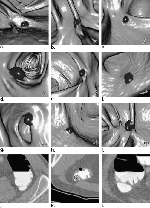
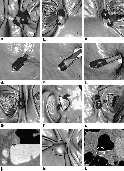
Fecal tagging computed tomographic colonography (ftCTC) reduces the discomfort and the inconvenience of patients associated with bowel cleansing procedures before CT scanning. In conventional colonic polyp detection techniques for ftCTC, a digital bowel cleansing (DBC) technique is applied to detect polyps in tagged fecal materials (TFM). However, DBC removes the surface of soft tissues and hampers polyp detection. We developed a colonic polyp detection method for CT colonographic examination that enables the detection of polyps surrounded by air and polyps surrounded by TFM without DBC.
Materials and Methods
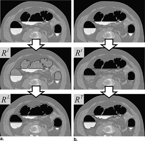
CT values inside the polyps surrounded by air and polyps surrounded by TFM tend to gradually increase (blob structure) and decrease (inverse-blob structure) from outward to inward, respectively. We developed blob and inverse-blob structure enhancement filters based on the eigenvalues of a Hessian matrix to detect polyps using their intensity characteristic. False-positive elimination is performed using three feature values: volume, maximum value of filter outputs, and standard deviation of CT values inside the polyp candidates.
Results
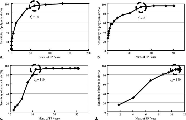
The proposed method is applied to 104 cases of ftCTC images that include 57 polyps larger than 6 mm in diameter. The sensitivity of the method was 91.2% (52/57) with 11.4 false positives per case.
Conclusions
The proposed method detects polyps with high sensitivity and 11.4 false positives per case without adverse effects on the DBC.
Colorectal cancer is the third most common cancer in the United States . Early detection and treatment of it can result in a complete cure. However, if the cancer is found in a later stage, a complete cure is quite difficult because of metastasis. Early detection of colonic cancer by screening is crucial. Currently, colonoscopy and barium enema are available for the screening of colorectal cancers. A colonoscopy is performed by inserting a colonoscope into the colon from the anus to examine the inside of the colon. The colonic wall is observed by colonoscope images to discover lesions. A barium enema is done using contrast agents containing barium. Before taking x-ray images, contrast agents are inserted into the anus. The contrast agents clearly show up in the colon on x-ray pictures. These inspection methods are expensive, and using a colonoscope may perforate the colon. Furthermore, these inspection procedures are complex and time-consuming. Therefore, when these methods are performed as screenings the loads on patients are a problem.
Computed tomographic colonography (CTC) or virtual colonoscopy is a new colon inspection method for examining the inside of the colon . The CTC system generates virtual colonoscopic views from abdominal computed tomographic (CT) images and enables physicians to freely observe inside the colon. Because physicians diagnose a virtualized human body reconstructed on a computer from the CT images of a patient, the load on a patient is greatly reduced by using CTC. Diagnosis using CTC is also less painful than previous inspection methods. However, the colon has many haustra and its shape is long and convoluted, and many blind areas are produced during diagnosis using CTC. About 30% of the colonic wall is unobserved during a fly-through along a centerline of the colon . To reduce the overlooked lesions existing in the blind areas, a physician has to repeatedly change the viewpoint and the viewing direction of the virtual camera of CTC. This task is time-consuming.
Get Radiology Tree app to read full this article<
 Open full size image
Figure 1
Example of colonic polyps surrounded by (a) air and (b) tagged fecal materials (TFM).
 Open full size image
Figure 2
Example of digital bowel cleansing (DBC) process applied to case shown in Figure 1 b. This image is obtained by changing computed tomographic (CT) values of high CT value voxels inside the colon to a CT value equivalent to air.
Get Radiology Tree app to read full this article<
Get Radiology Tree app to read full this article<
Materials and methods
Overview
Get Radiology Tree app to read full this article<
Preprocessing
Get Radiology Tree app to read full this article<
Get Radiology Tree app to read full this article<
Polyp Detection
Calculation of Hessian Matrix
Get Radiology Tree app to read full this article<
f(x,y,z;a)=a1x2+a2y2+a3z2+a4xy+a5yz+a6zx+a7x+a8y+a9z+a10, f
(
x
,
y
,
z
;
a
)
=
a
1
x
2
+
a
2
y
2
+
a
3
z
2
+
a
4
x
y
+
a
5
y
z
+
a
6
z
x
+
a
7
x
+
a
8
y
+
a
9
z
+
a
10
,
where a is a coefficient vector described as a=(a1,…,a10) a
=
(
a
1
,
…
,
a
10
) . To approximate CT values in a local region at voxel (i,j,k) (
i
,
j
,
k
) , we need to obtain vector a that minimizes square error εi,j,k ε
i
,
j
,
k , defined by
εi,j,k=∑p,q,r{gp,q,r−f(p,q,r;a)}2 ε
i
,
j
,
k
=
∑
p
,
q
,
r
{
g
p
,
q
,
r
−
f
(
p
,
q
,
r
;
a
)
}
2
where (p,q,r) (
p
,
q
,
r
) is a position on a local coordinate system in the local area. gp,q,r g
p
,
q
,
r is a CT value of voxel (p,q,r) (
p
,
q
,
r
) . To obtain a that minimizes εi,j,k ε
i
,
j
,
k , we need to solve the system of equations:
∂εi,j,k∂am=−2∂f∂am∑p,q,r{gp,q,r−f(p,q,r;a)}=0, ∂
ε
i
,
j
,
k
∂
a
m
=
−
2
∂
f
∂
a
m
∑
p
,
q
,
r
{
g
p
,
q
,
r
−
f
(
p
,
q
,
r
;
a
)
}
=
0
,
where m=1,2,…,10 m
=
1
,
2
,
…
,
10 . Polynomial f(x,y,z;a) f
(
x
,
y
,
z
;
a
) is obtained by the method described previously. We obtain Hessian matrix H consisting of second-order partial differential coefficients of f :
H=⎡⎣⎢⎢⎢⎢⎢⎢⎢∂2f∂x2∣∣(i,j,k)∂2f∂y∂x∣∣(i,j,k)∂2f∂z∂x∣∣(i,j,k)∂2f∂x∂y∣∣(i,j,k)∂2f∂y2∣∣(i,j,k)∂2f∂z∂y∣∣(i,j,k)∂2f∂x∂z∣∣(i,j,k)∂2f∂y∂z∣∣(i,j,k)∂2f∂z2∣∣(i,j,k)⎤⎦⎥⎥⎥⎥⎥⎥⎥. H
=
[
∂
2
f
∂
x
2
|
(
i
,
j
,
k
)
∂
2
f
∂
x
∂
y
|
(
i
,
j
,
k
)
∂
2
f
∂
x
∂
z
|
(
i
,
j
,
k
)
∂
2
f
∂
y
∂
x
|
(
i
,
j
,
k
)
∂
2
f
∂
y
2
|
(
i
,
j
,
k
)
∂
2
f
∂
y
∂
z
|
(
i
,
j
,
k
)
∂
2
f
∂
z
∂
x
|
(
i
,
j
,
k
)
∂
2
f
∂
z
∂
y
|
(
i
,
j
,
k
)
∂
2
f
∂
z
2
|
(
i
,
j
,
k
)
]
.
Get Radiology Tree app to read full this article<
Detection in Air Regions by a Blob Structure Enhancement Filter
Get Radiology Tree app to read full this article<
Get Radiology Tree app to read full this article<
SL(λ1,λ2,λ3)=⎧⎩⎨⌊λ21λˆ⌋0if0>λ1,λ2,λ3,otherwise, S
L
(
λ
1
,
λ
2
,
λ
3
)
=
{
⌊
λ
1
2
λ
ˆ
⌋
i
f
0
λ
1
,
λ
2
,
λ
3
,
0
otherwise
,
where λˆ=|λ1+λ2+λ3|/3 λ
ˆ
=
|
λ
1
+
λ
2
+
λ
3
|
/
3 . Equation 5 outputs a high value for 0»λ1 0
λ
1 and λ1≅λˆ λ
1
≅
λ
ˆ . In contrast, it outputs a low value for λ1≅0 λ
1
≅
0 or λˆ»λ1 λ
ˆ
λ
1 . Equation 5 outputs a high value when the absolute values of λ 1 , λ 2 , and λ 3 are high and subequal. We generate a blob structure enhanced image I l (a grayscale image with background voxels) that has output values of S L on each voxel. Polyp candidate regions are extracted as a set of voxels whose values are greater than 0 in I l .
Get Radiology Tree app to read full this article<
Detection in TFM Regions by an Inverse-blob Structure Enhancement Filter
Get Radiology Tree app to read full this article<
Get Radiology Tree app to read full this article<
ST(λ1,λ2,λ3)=⎧⎩⎨⌊λ21λˆ⌋0if0<λ1,λ2,λ3,otherwise. S
T
(
λ
1
,
λ
2
,
λ
3
)
=
{
⌊
λ
1
2
λ
ˆ
⌋
i
f
0
<
λ
1
,
λ
2
,
λ
3
,
0
otherwise
.
Get Radiology Tree app to read full this article<
Get Radiology Tree app to read full this article<
False-positive Elimination
Get Radiology Tree app to read full this article<
Small Component Elimination
Get Radiology Tree app to read full this article<
Low-value Component Elimination
Get Radiology Tree app to read full this article<
Elimination Using a Standard Deviation of CT Values
Get Radiology Tree app to read full this article<
Results
Get Radiology Tree app to read full this article<
Table 1
Acquisition Parameters of Fecal Tagging Computed Tomographic Colonography Images
Image size 512 × 512 pixels Number of slices 283–551 Pixel spacing 0.55–0.76 mm Slice spacing 1.00 mm Slice thickness 1.25 mm
Get Radiology Tree app to read full this article<
Get Radiology Tree app to read full this article<
Get Radiology Tree app to read full this article<
Get Radiology Tree app to read full this article<
Get Radiology Tree app to read full this article<
Discussion
Get Radiology Tree app to read full this article<
Get Radiology Tree app to read full this article<
Get Radiology Tree app to read full this article<
Conclusion
Get Radiology Tree app to read full this article<
Acknowledgments
Get Radiology Tree app to read full this article<
Get Radiology Tree app to read full this article<
References
1. ACS Cancer facts and figures 2007. American Cancer Society, 2007. Available at: http://www.cancer.org/downloads/STT/CAFF2007PWSecured.pdf .
2. Yoshida H.: Three-dimensional computer-aided diagnosis in CT colonography. Multidimensional Image Processing, Analysis, and Display: RSNA Categorical Course in Diagnostic. Radiology Physics 2005; pp. 237-251.
3. Hayashi Y., Mori K., Suenaga Y., et. al.: A method for detecting undisplayed regions in virtual colonoscopy and its application to quantitative evaluation of fly-through methods. Acad Radiol 2003; 10: pp. 1380-1391.
4. Yao J., Miller M., Franaszek M., et. al.: Colonic polyp segmentation in CT colonography-based on fuzzy clustering and deformable models. IEEE Trans Med Imaging 2004; 23: pp. 1344-1352.
5. Huang A., Summers R.M., Hara A.K.: Surface curvature estimation for automatic colonic polyp detection. Proc SPIE Med Imaging 2005; 5746: pp. 393-400.
6. Nappi J., Yoshida H.: Feature-guided analysis for reduction of false positives in CAD of polyps for computed tomographic colonography. Med Phys 2003; 30: pp. 1592-1601.
7. Nappi J., Yoshida H.: Fully automated three-dimensional detection of polyps in fecal-tagging CT colonography. Acad Radiol 2007; 14: pp. 287-300.
8. Kitasaka T., Mori K., Kimura T., et. al.: A method for detecting colonic polyps using curve fitting from 3D abdominal CT images. Proc SPIE Med Imaging 2005; 5746: pp. 403-414.
9. Jerebko A., Lakare S., Cathier P., et. al.: Symmetric curvature patterns for colonic polyp detection. MICCAI 2006; 4191: pp. 169-176.
10. Lee J., Kim J., Kim S., et. al.: Fine tuning of internal parameters of Hessian-based polyp detection scheme for CT colonography CAD. Int J CARS 2007; 2: pp. S518.
11. Kim S., Lee J., Lee J., et. al.: Computer-aided detection of colonic polyps at CT colonography using a Hessian matrix-based algorithm: preliminary study. AJR Am J Roentgenol 2007; 189: pp. 41-51.
12. Cai W., Nappi J., Zalis M., et. al.: Digital bowel cleansing for computer-aided detection of polyps in fecal-tagging CT colonography. Proc SPIE Med Imaging 2006; 6144: pp. 614422.
13. Yoshida H., Nappi J.: CAD in CT colonography without and with oral contrast agents: progress and challenges. Comput Med Imag Graphic 2007; 31: pp. 267-284.
14. Summers R.M., Franaszek M., Miller M.T., et. al.: Computer-aided detection of polyps on oral contrast-enhanced CT colonography. AJR Am J Roentgenol 2005; 184: pp. 105-108.
15. Sato Y., Westin C., Bhalerao A., et. al.: Tissue classification based on 3D local intensity structures for volume rendering. IEEE Trans Visualization Comp Graphics 2000; 6: pp. 160-180.
16. Fidler J, Johnson C. Flat polyps of the colon: accuracy of detection by CT colonography and histologic significance. Abdom Imaging 2008; PMID 18414934. (Epub ahead of print)
17. Takayama T., Sato Y., Sagawa T., et. al.: Application of polypectomy and high risk groups for recurrence of post-polypectomy. [in Japanese] Gastroenterology 2004; 39: pp. 258-263.