Dynamic Contrast-Enhanced MRI Kinetic Parameters as Prognostic Biomarkers for Prediction of Survival of Patient with Advanced Hepatocellular Carcinoma

Rationale and Objectives

Tracer kinetic model selection for dynamic contrast-enhanced magnetic resonance imaging (DCE-MRI) data analysis influences its use as a prognostic biomarker. Our aim was to find DCE-MRI parameters that predict 1-year survival (1YS) and overall survival (OS) among patients with advanced hepatocellular carcinoma (HCC) treated with antiangiogenic monotherapy by conducting a proof-of-concept comparative study of five different kinetic models.

Materials and Methods

Twenty patients with advanced HCC underwent DCE-MRI and subsequently received sunitinib. Pretreatment DCE-MRI data were analyzed retrospectively by using the Tofts-Kety (TK), extended TK, two compartment exchange, adiabatic approximation to the tissue homogeneity (AATH), and distributed parameter (DP) models. Arterial flow fraction ( γ ), arterial blood flow ( BF A ), permeability–surface area product ( PS ), fractional interstitial volume ( v I ), and other five parameters were calculated for each model. Individual parameters were evaluated for 1YS prediction using cross-validated Kaplan–Meier analysis, and for association with OS using univariate Cox regression analysis, with additional permutation testing.

Results

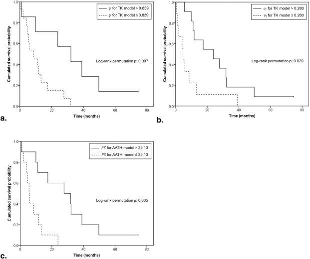
For 1YS prediction, the TK model–derived γ ( P = .007) and v I ( P = .029) and the AATH model-derived PS ( P = .005) were significant; all these parameters were lower in the high-risk group. Increase in the AATH model-derived PS and the DP model-derived BF A was associated with significant increase in OS with hazard ratios of 0.766 ( P = .023) and 0.809 ( P = .025), respectively.

Conclusions

The AATH model-derived PS was an effective prognostic biomarker for both 1YS and OS.

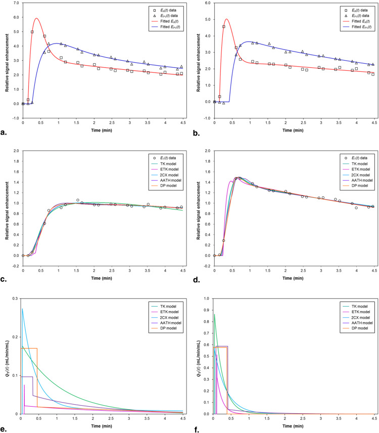
Dynamic contrast-enhanced magnetic resonance imaging (DCE-MRI) enables tumor vascular physiology to be assessed and has a potential role in monitoring the response of hepatocellular carcinoma (HCC) to systemic therapy . Assessment of hemodynamic changes in the liver is especially challenging because of dual blood supply to this organ . HCC is a highly vascularized tumor that draws the majority of its blood supply from branches of the hepatic artery . Nevertheless, accurate quantification of the proportions of the blood supply to HCC from the hepatic arterial and the portal venous system in vivo may be of clinical value for diagnosis and treatment. Indeed, dual-input tracer kinetic models for DCE-MRI have become important for quantitative analysis of hepatic perfusion .

To date, there has been no effort to seek data comparing the relative performance of different tracer kinetic models for DCE-MRI in predicting survival of patients with advanced HCC. Previous DCE-MRI studies for the liver have mainly used either a dual-input single-compartment model or a dual-input two-compartment distributed parameter (DP) model . There exist a variety of other tracer kinetic models with different physiological scenarios ; thus, it is difficult to select an optimal model that describes the clinical outcome of interest without comparing the diagnostic or prognostic efficacy of these models . Because HCC is a heterogeneous tumor, comparing different kinetic models with varying degrees of complexity is of central importance and raises the possibility of finding effective biomarkers for improved diagnosis, prognosis, and treatment of HCC.

Get Radiology Tree app to read full this article<

Materials and methods

Patients

Get Radiology Tree app to read full this article<

DCE-MRI Protocol

Get Radiology Tree app to read full this article<

Image Analysis

Get Radiology Tree app to read full this article<

Table 1

Symbols and Definitions for Kinetic Parameters

Term Definition Unit of Measure_C_ A Arterial blood concentration of tracer g/mL_C_ PV Portal blood concentration of tracer g/mL_C_ P Concentration of tracer in the plasma compartment g/mL_C_ I Concentration of tracer in the interstitial compartment g/mL_C_ T Concentration of tracer in tissue g/mL_E_ A Relative signal enhancement in artery None_E_ PV Relative signal enhancement in portal vein None_E_ T Relative signal enhancement in tissue None_R_ T Tissue residue function None_Q_ T Impulse response function of the tissue mL/min/mL_F_ Total hepatic plasma flow mL/min_γ_ Arterial flow fraction None_F_ A Arterial plasma flow mL/min_F_ PV Portal plasma flow mL/min_BF_ Total hepatic blood flow mL/min/100 g_BF_ A Arterial blood flow mL/min/100 g_BF_ PV Portal blood flow mL/min/100 g_BV_ Blood volume mL/100 g_MTT_ Mean transit time min_PS_ Permeability–surface area product mL/min (or mL/min/100 g)v P Fractional plasma volume None_v_ I Fractional interstitial volume None_E_ Extraction fraction None_H_ LV Hematocrit in major (large) vessels None_H_ SV Hematocrit in small vessels None_m_ Tissue mass g_ρ_ T Tissue density g/cm 3 V P Volume of the plasma compartment mL_V_ I Volume of the interstitial compartment mL_V_ T Tissue volume mLF/VT F

T Total hepatic perfusion mL/min/mLFA/VT F

T Arterial perfusion mL/min/mLFPV/VT F

T Portal perfusion mL/min/mLKTrans=EF/VT K

Trans

T Volume transfer constant between the plasma and interstitial compartments mL/min/mLVP/F V

F Capillary transit time minVP/PS V

S Capillary leakage time min_t_ Lag,T Difference in bolus arrival time between C A (or C PV ) and C T min

Get Radiology Tree app to read full this article<

Treatment and Follow-up

Get Radiology Tree app to read full this article<

Statistical Analysis

Get Radiology Tree app to read full this article<

Results

Get Radiology Tree app to read full this article<

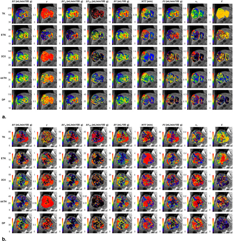
$Figure 2, Parametric maps of total hepatic blood flow ( BF ), arterial flow fraction ( γ ), arterial blood flow ( BF A ), portal blood flow ( BF PV ), blood volume ( BV ), mean transit time ( MTT ), permeability–surface area product ( PS ), fractional interstitial volume ( v I ), and extraction fraction ( E ) for HCC in (a) a low-risk man aged 52 years who survived 23.87 months and (b) a high-risk man aged 72 years who survived 8.53 months. AATH, adiabatic approximation to the tissue homogeneity; DP = distributed parameter; ETK, extended Tofts-Kety; HCC, hepatocellular carcinoma; TK, Tofts-Kety; 2CX, two-compartmental exchange. (Color version of figure is available online.)$

Table 2

Parameter Values Derived From the Five Different Kinetic Models

Parameter Mean ± SD TK ETK 2CX AATH DP_BF_ 156.6 ± 96.40 39.97 ± 21.13 66.86 ± 34.43 45.41 ± 21.59 59.52 ± 27.17γ 0.655 ± 0.280 0.381 ± 0.217 0.713 ± 0.304 0.574 ± 0.263 0.512 ± 0.287BF A 105.7 ± 89.75 16.59 ± 14.20 50.68 ± 36.74 26.09 ± 18.45 31.85 ± 24.19BF PV 50.87 ± 49.16 23.38 ± 13.27 16.18 ± 19.39 19.32 ± 16.03 27.66 ± 19.23BV 54.15 ± 30.82 20.83 ± 10.26 24.69 ± 11.10 16.83 ± 7.968 24.19 ± 10.51MTT 1.461 ± 2.404 4.442 ± 1.964 1.917 ± 2.147 2.008 ± 2.237 2.061 ± 2.400PS 116.4 ± 73.39 34.06 ± 24.52 42.48 ± 29.32 21.54 ± 17.29 6.495 ± 4.756v I 0.274 ± 0.082 0.201 ± 0.082 0.231 ± 0.141 0.273 ± 0.197 0.280 ± 0.076E 0.617 ± 0.074 0.649 ± 0.124 0.391 ± 0.134 0.376 ± 0.179 0.147 ± 0.108RMSE 0.181 ± 0.129 0.141 ± 0.091 0.175 ± 0.135 0.212 ± 0.217 0.162 ± 0.129

AATH, adiabatic approximation to the tissue homogeneity; BF , total hepatic blood flow (in mL/min/100 g); BF A , arterial blood flow (in mL/min/100 g); BF PV , portal blood flow (in mL/min/100 g); BV , blood volume (in mL/100 g); DP, distributed parameter; E , extraction fraction (unitless); ETK, extended Tofts-Kety; MTT , mean transit time (in min); PS , permeability–surface area product (in mL/min/100 g); RMSE , root-mean-square error; SD, standard deviation; TK, Tofts-Kety; v I , fractional interstitial volume (unitless); γ , arterial flow fraction (unitless); 2CX, two compartment exchange.

Get Radiology Tree app to read full this article<

Kaplan–Meier Survival Analysis

Get Radiology Tree app to read full this article<

Table 3

Optimal Cutoff Values of Parameters and Their Log-Rank Test Results From Leave-One-Out Cross-validated Kaplan–Meier Analysis with Respect to 1-Year Survival

Parameter Cutoff Value ( P Value) TK ETK 2CX AATH DP_BF_ 120.1 (.589) 45.70 (.216) 63.99 (.423) 33.81 (.874) 68.05 (.682)γ 0.839 ( .007 )* 0.331 (.634) 0.649 (.304) 0.603 (.681) 0.515 (.305)BF A 53.60 (.767) 11.59 (.450) 52.88 (.133) 17.14 (.660) 24.00 (.229)BF PV 22.30 (.422) 25.91 (.797) 9.548 (.472) 10.24 (.272) 18.50 (.234)BV 40.09 (.479) 14.30 (.815) 21.18 (.720) 11.88 (.874) 19.66 (.487)MTT 0.318 (.329) 5.111 (.471) 1.026 (.426) 1.186 (.329) 1.198 (.515)PS 85.38 (.345) 35.03 (.315) 33.61 (.574) 25.13 ( .005 )* 2.798 (.855)v I 0.280 ( .029 )* 0.188 (.337) 0.221 (.565) 0.211 (.296) 0.242 (.737)E 0.605 (.999) 0.580 (.502) 0.378 (.361) 0.416 (.288) 0.109 (.658)

AATH, adiabatic approximation to the tissue homogeneity; BF , total hepatic blood flow (in mL/min/100 g); BF A , arterial blood flow (in mL/min/100 g); BF PV , portal blood flow (in mL/min/100 g); BV , blood volume (in mL/100 g); DP, distributed parameter; E , extraction fraction (unitless); ETK, extended Tofts-Kety; MTT , mean transit time (in min); PS , permeability–surface area product (in mL/min/100 g); TK, Tofts-Kety; v I , fractional interstitial volume (unitless); γ , arterial flow fraction (unitless); 2CX, two compartment exchange.

Bold numbers with asterisk (*) indicate a statistically significant difference in the 1000 log-rank permutation test (two-sided P < .05).

$Figure 3, Leave-one-out cross-validated Kaplan–Meier plots for (a) arterial flow fraction ( γ ) and (b) fractional interstitial volume ( v I ) derived from the Tofts-Kety (TK) model and (c) permeability–surface area product ( PS ) derived from the adiabatic approximation to the tissue homogeneity (AATH) model. Survival in advanced HCC patients treated with sunitinib was better with γ over 0.839 and v I over 0.280 in the TK model and with PS over 25.13 mL/min/100 g in the AATH model, respectively. HCC, hepatocellular carcinoma.$

Get Radiology Tree app to read full this article<

Cox Proportional Hazard Model

Get Radiology Tree app to read full this article<

Table 4

Results From Univariate Cox Proportional Hazards Regression Analysis of Parameters with Respect to Overall Survival

Parameter Hazard Ratio ( P Value) TK ETK 2CX AATH DP_BF_ 0.816 (.375) 0.750 (0.208) 0.745 (.101) 0.826 (.492) 0.730 (.240)γ 0.824 (.359) 0.795 (0.305) 0.929 (.650) 0.855 (.364) 0.806 (.079)BF A 0.798 (.059) 0.829 (.085) 0.826 (.068) 0.843 (.268) 0.809 ( .025 )*BF PV 1.227 (.149) 0.798 (.349) 1.032 (.756) 0.981 (.865) 1.175 (.343)BV 0.862 (.558) 0.741 (.327) 0.646 (.134) 0.779 (.394) 0.762 (.353)MTT 1.229 (.166) 0.848 (.671) 1.370 (.113) 1.196 (.406) 1.215 (.391)PS 0.867 (.505) 0.838 (.387) 0.762 (.223) 0.766 ( .023 )* 0.948 (.731)v I 0.494 (.141) 0.679 (.349) 1.079 (.605) 1.222 (.528) 0.664 (.510)E 4.884 (.448) 1.437 (.689) 0.867 (.796) 0.790 (.059) 1.069 (.680)

AATH, adiabatic approximation to the tissue homogeneity; BF , total hepatic blood flow (in mL/min/100 g); BF A , arterial blood flow (in mL/min/100 g); BF PV , portal blood flow (in mL/min/100 g); BV , blood volume (in mL/100 g); DP, distributed parameter; E , extraction fraction (unitless); ETK, extended Tofts-Kety; MTT , mean transit time (in min); PS , permeability–surface area product (in mL/min/100 g); TK, Tofts-Kety; v I , fractional interstitial volume (unitless); γ , arterial flow fraction (unitless); 2CX, two compartment exchange.

Bold numbers with asterisk (*) indicate a statistically significant difference in the 1000 permutation test for hazard ratio in univariate Cox proportional hazards analysis (two-sided P < .05).

Get Radiology Tree app to read full this article<

Discussion

Get Radiology Tree app to read full this article<

Appendix

Get Radiology Tree app to read full this article<

CA(t)=aB,A(t−tLag,A1)e−μB,A(t−tLag,A1)u(t−tLag,A1)−aB,AaG,AμB,A−μG,A{(t−tLag,A1−tLag,A2)e−μB,A(t−tLag,A1−tLag,A2)−e−μG,A(t−tLag,A1−tLag,A2)−e−μB,A(t−tLag,A1−tLag,A2)μB,A−μG,A}u(t−tLag,A1−tLag,A2), C

(

)

B,A

(

−

Lag,A

)

−

B,A

(

−

Lag,A

)

(

−

Lag,A

)

−

B,A

G,A

B,A

−

G,A

{

(

−

Lag,A

−

Lag,A

)

−

B,A

(

−

Lag,A

−

Lag,A

)

−

G,A

(

−

Lag,A

−

Lag,A

)

−

B,A

(

−

Lag,A

−

Lag,A

)

B,A

−

G,A

}

(

−

Lag,A

−

Lag,A

)

Get Radiology Tree app to read full this article<

CPV(t)=aB,PV(t−tLag,PV1)e−μB,PV(t−tLag,PV1)u(t−tLag,PV1)−aB,PVaG,PVμB,PV−μG,PV{(t−tLag,PV1−tLag,PV2)e−μB,PV(t−tLag,PV1−tLag,PV2)−e−μG,PV(t−tLag,PV1−tLag,PV2)−e−μB,PV(t−tLag,PV1−tLag,PV2)μB,PV−μG,PV}u(t−tLag,PV1−tLag,PV2), C

(

)

B,PV

(

−

Lag,PV

)

−

B,PV

(

−

Lag,PV

)

(

−

Lag,PV

)

−

B,PV

G,PV

B,PV

−

G,PV

{

(

−

Lag,PV

−

Lag,PV

)

−

B,PV

(

−

Lag,PV

−

Lag,PV

)

−

G,PV

(

−

Lag,PV

−

Lag,PV

)

−

B,PV

(

−

Lag,PV

−

Lag,PV

)

B,PV

−

G,PV

}

(

−

Lag,PV

−

Lag,PV

)

where u(t) u

(

) is the unit step function.

Get Radiology Tree app to read full this article<

CT(t)=RT(t−tLag,T)⊗(FA/VT)CA(t)+(FPV/VT)CPV(t)1−HLV=FVTRT(t−tLag,T)⊗γCA(t)+(1−γ)CPV(t)1−HLV=QT(t−tLag,T)⊗γCA(t)+(1−γ)CPV(t)1−HLV, C

(

)

(

−

Lag,T

)

⊗

(

)

(

)

(

)

(

)

−

(

−

Lag,T

)

⊗

(

)

(

−

)

(

)

−

(

−

Lag,T

)

⊗

(

)

(

−

)

(

)

−

where HLV H

LV is the hematocrit of blood in large vessels ( ≅0.45 ≅

45 ) for estimation of the input tracer concentration in blood plasma , and VT,F/VT,FA/VT,FPV/VT,tLag,T,RT(t) V

Lag,T

(

) , and QT(t) Q

(

) are kinetic parameters and functions as defined in Table 1. The fundamental assumption behind Equation (A2) is that tracer transport within the capillary-tissue system can be modeled as a linear and time-invariant (stationary) system. All models considered in this study fall under this assumption. All five models are derived from their own tissue residue function RT(t) R

(

) . To account for the difference in bolus arrival times between the feeding vessels (ie, hepatic artery and portal vein) and the liver tissue, a time lag (delay) to the liver tissue, tLag,T t

Lag,T , can be imposed on either the net input function (ie, CA(t) C

(

) and CPV(t) C

(

) ) or RT(t) R

(

) for calculation of CT(t) C

(

) . The analytic solution of CT(t) C

(

) for each model can be derived by incorporating Equations (A1a) and (A1b) into Equation (A2) .

Get Radiology Tree app to read full this article<

dCP(t)dt=FVP[γCA(t−tLag,T)+(1−γ)CPV(t−tLag,T)1−HLV−CP(t)]−PSVP[CP(t)−CI(t)], d

(

)

[

(

−

Lag,T

)

(

−

)

(

−

Lag,T

)

−

(

)

]

−

[

(

)

−

(

)

]

Get Radiology Tree app to read full this article<

dCI(t)dt=PSVI[CP(t)−CI(t)], d

(

)

[

(

)

−

(

)

]

where PS , V P , V I , C P , and C I are defined as in Table 1. The total tissue concentration of the 2CX model is given by CT(t)=vpCp(t)+v1C1(t) C

(

)

(

)

(

) , where vP=VP/VT v

T and vI=VI/VT v

T . Thus, the solution of the tissue residue function of the 2CX model, RT,2CX(t) R

(

) , is given by:

RT,2CX(t)=Aeαt+(1−A)eβt, R

(

)

(

−

)

Get Radiology Tree app to read full this article<

(αβ)=12[−{FVP+(1+vPvI)PSVP}±{FVP+(1+vPvI)PSVP}2−4vPvIFVPPSVP−−−−−−−−−−−−−−−−−−−−−−−−−−−√], (

)

[

−

{

(

)

}

{

(

)

}

−

]

Get Radiology Tree app to read full this article<

A=α+(1+vPvI)PSVPα−β. A

(

)

−

Get Radiology Tree app to read full this article<

CT,2CX(t)=FVT(11−HLV)[γ{(KA1eαtA1+KA2eβtA1+KA3e−μB,AtA1+KA4tA1e−μB,AtA1)u(tA1)+(KA5eαtA2+KA6eβtA2+KA7e−μB,AtA2+KA8e−μG,AtA2+KA9tA2e−μB,AtA2)u(tA2)}+(1−γ){(KPV1eαtPV1+KPV2eβtPV1+KPV3e−μB,PVtPV1+KPV4tPV1e−μB,PVtPV1)u(tPV1)+(KPV5eαtPV2+KPV6eβtPV2+KPV7e−μB,PVtPV2+KPV8e−μG,PVtPV2+KPV9tPV2e−μB,PVtPV2)u(tPV2)}], C

(

)

(

−

)

[

{

(

−

B,A

−

B,A

)

(

)

(

−

B,A

−

G,A

−

B,A

)

(

)

}

(

−

)

{

(

−

)

(

)

(

−

)

(

)

}

]

where tA1=t−tLag,A1−tLag,T t

−

Lag,A

−

Lag,T , tA2=tA1−tLag,A2 t

−

Lag

2 , tPV1=t−tLag,PV1−tLag,T t

−

Lag,PV

−

Lag,T , tPV2=tPV1−tLag,PV2 t

−

Lag,PV

2 , KA1=AaB,A/(α+μB,A)2 K

B,A

(

B,A

)

2 , KA2=(1−A)aB,A/(β+μB,A)2 K

(

−

)

B,A

(

B,A

)

2 , KA3=−(KA1+KA2) K

−

(

) , KA4=−{KA1(α+μB,A)+KA2(β+μB,A)} K

−

{

(

B,A

)

(

B,A

)

} , KA5=KA1aG,A/(α+μG,A) K

G,A

(

G,A

) , KA6=KA2aG,A/(β+μG,A) K

G,A

(

G,A

) , KA7={aG,A/(μB,A−μG,A)2}{KA1(α+2μB,A−μG,A)+KA2(β+2μB,A−μG,A)} K

{

(

B,A

−

G,A

)

}

{

(

B,A

−

G,A

)

(

B,A

−

G,A

)

} , KA8=−{aB,A/(μB,A−μG,A)2}{A(KA5/KA1)+(1−A)(KA6/KA2)} K

−

{

B,A

(

B,A

−

G,A

)

}

{

(

)

(

−

)

(

)

} , KA9=−KA4aG,A/(μB,A−μG,A) K

−

G,A

(

B,A

−

G,A

) , KPV1=AaB,PV/(α+μB,PV)2 K

B,PV

(

B,PV

)

2 , KPV2=(1−A)aB,PV/(β+μB,PV)2 K

(

−

)

B,PV

(

B,PV

)

2 , KPV3=−(KPV1+KPV2) K

−

(

) , KPV4=−{KPV1(α+μB,PV)+KPV2(β+μB,PV)} K

−

{

(

B,PV

)

(

B,PV

)

} , KPV5=KPV1aG,PV/(α+μG,PV) K

G,PV

(

G,PV

) , KPV6=KPV2aG,PV/(β+μG,PV) K

G,PV

(

G,PV

) , KPV7={aG,PV/(μB,PV−μG,PV)2}{KPV1(α+2μB,PV−μG,PV)+KPV2(β+2μB,PV−μG,PV)} K

{

G,PV

(

B,PV

−

G,PV

)

}

{

(

B,PV

−

G,PV

)

(

B,PV

−

G,PV

)

} , KPV8=−{aB,PV/(μB,PV−μG,PV)2}{A(KPV5/KPV1)+(1−A)(KPV6/KPV2)} K

−

{

B,PV

(

B,PV

−

G,PV

)

}

{

(

)

(

−

)

(

)

} , and KPV9=−KPV4aG,PV/(μB,PV−μG,PV) K

−

G,PV

(

B,PV

−

G,PV

) .

Get Radiology Tree app to read full this article<

∂CP(x,t)∂t=FVP[{γCA(t−tLag,T)+(1−γ)CPV(t−tLag,T)}δ(x)1−HLV−L∂CP(x,t)∂x]−PSVP[CP(x,t)−CI(t)], ∂

(

)

∂

[

{

(

−

Lag,T

)

(

−

)

(

−

Lag,T

)

}

(

)

−

∂

(

)

∂

]

−

[

(

)

−

(

)

]

Get Radiology Tree app to read full this article<

dCI(t)dt=1LPSVI∫0L[CP(x,t)−CI(t)]dx, d

(

)

∫

[

(

)

−

(

)

]

where δ(x) δ

(

) is the Dirac delta function that denotes the idealized impulse excitation of a unit-mass source at x = 0. It should be noted that there exists no known closed-form solution for the system of Equations (A7a) and (A7b) in the time domain.

Get Radiology Tree app to read full this article<

∂CP(x,t)∂t=FVP[{γCA(t−tLag,T)+(1−γ)CPV(t−tLag,T)}δ(x)1−HLV−L∂CP(x,t)∂x], ∂

(

)

∂

[

{

(

−

Lag,T

)

(

−

)

(

−

Lag,T

)

}

(

)

−

∂

(

)

∂

]

Get Radiology Tree app to read full this article<

dCI(t)dt=EFVI[CP(L,t)−CI(t)]. d

(

)

[

(

)

−

(

)

]

Get Radiology Tree app to read full this article<

RT,AATH(t)=u(t)+[Ee−vPEFvIVP(t−VPF)−1]u(t−VPF). R

T,AATH

(

)

(

)

[

−

(

−

)

−

]

(

−

)

Get Radiology Tree app to read full this article<

CT,AATH(t)=FVT(11−HLV)[γ[{LA1(1−e−μB,AtA1)+LA2tA1e−μB,AtA1}u(tA1)+(LA3+LA4e−μB,AtA2+LA5e−μG,AtA2−LA2tA2e−μB,AtA2)u(tA2)+{LA6e−vPEFvIVP(tA1−VPF)−LA1+LA7e−μB,A(tA1−VPF)+LA8(tA1−VPF)e−μB,A(tA1−VPF)}u(tA1−VPF)+{LA9evPEFvIVP(tA2−VPF)−LA3+LA10e−μB,A(tA2−VPF)+LA11e−μG,A(tA2−VPF)+LA12(tA2−VPF)e−μB,A(tA2−VPF)}u(tA2−VPF)]+(1−γ)[{LPV1(1−e−μB,PVtPV1)+LPV2tPV1e−μB,PVtPV1}u(tPV1)+(LPV3+LPV4e−μB,PVtPV2+LPV5e−μG,PVtPV2−LPV2tPV2e−μB,PVtPV2)u(tPV2)+{LPV6e−vPEFvIVP(tPV1−VPF)−LPV1+LPV7e−μB,PV(tPV1−VPF)+LPV8(tPV1−VPF)e−μB,PV(tPV1−VPF)}u(tPV1−VPF)+{LPV9e−vPEFvIVP(tPV2−VPF)−LPV3+LPV10e−μB,PV(tPV2−VPF)+LPV11e−μG,PV(tPV2−VPF)+LPV12(tPV2−VPF)e−μB,PV(tPV2−VPF)}u(tPV2−VPF)]], C

T,AATH

(

)

(

−

)

[

{

(

−

B,A

)

−

B,A

}

(

)

(

−

B,A

−

G,A

−

B,A

)

(

)

{

−

(

−

)

−

B,A

(

−

)

(

−

)

−

(

−

)

}

(

−

)

{

(

−

)

−

B,A

(

−

)

−

G,A

(

−

)

(

−

)

−

B,A

(

−

)

}

(

−

)

]

(

−

)

[

{

(

−

B,PV

)

−

B,PV

}

(

)

(

−

B,PV

−

G,PV

−

B,PV

)

(

)

{

−

(

−

)

−

B,PV

(

−

)

(

−

)

−

B,PV

(

−

)

}

(

−

)

{

−

(

−

)

−

B,PV

(

−

)

−

G,PV

(

−

)

(

−

)

−

B,PV

(

−

)

}

(

−

)

]

where LA1=aB,A/(μB,A)2 L

B,A

(

B,A

)

2 , LA2=−LA1aG,AμB,A/(μB,A−μG,A) L

−

G,A

B,A

(

B,A

−

G,A

) , LA3=LA1(aG,A/μG,A) L

(

G,A

) , LA4=−LA2(2−μG,A/μB,A)/(μB,A−μG,A) L

−

(

−

G,A

B,A

)

(

B,A

−

G,A

) , LA5=−LA2(μB,A/μG,A)/(μB,A−μG,A) L

−

(

B,A

G,A

)

(

B,A

−

G,A

) , LA6=EaB,A/(μB,A−L1)2 L

B,A

(

B,A

−

)

2 , LA7=LA1−LA6 L

−

6 , LA8=LA1μB,A−LA6(μB,A−L1) L

B,A

−

(

B,A

−

) , LA9=LA6aG,A/(μG,A−L1) L

G,A

(

G,A

−

) , LA10=LA6{aG,A/(μB,A−μG,A)}{1+(μB,A−L1)/(μB,A−μG,A)}−LA4 L

{

G,A

(

B,A

−

G,A

)

}

{

(

B,A

−

)

(

B,A

−

G,A

)

}

−

4 , LA11=−LA2{μB,A/(μB,A−μG,A)}{1/μG,A−E/(μG,A−L1)} L

−

{

B,A

(

B,A

−

G,A

)

}

{

G,A

−

(

G,A

−

)

} , LA12=LA2μB,A{1/μB,A−E/(μB,A−L1)} L

B,A

{

B,A

−

(

B,A

−

)

} , LPV1=aB,PV/(μB,PV)2 L

B,PV

(

B,PV

)

2 , LPV2=−LPV1aG,PVμB,PV/(μB,PV−μG,PV) L

−

G,PV

B,PV

(

B,PV

−

G,PV

) , LPV3=LPV1(aG,PV/μG,PV) L

(

G,PV

) , LPV4=−LPV2(2−μG,PV/μB,PV)/(μB,PV−μG,PV) L

−

(

−

G,PV

B,PV

)

(

B,PV

−

G,PV

) , LPV5=−LPV2(μB,PV/μG,PV)/(μB,PV−μG,PV) L

−

(

B,PV

G,PV

)

(

B,PV

−

G,PV

) , LPV6=EaB,PV/(μB,PV−L1)2 L

B,PV

(

B,PV

−

)

2 , LPV7=LPV1−LPV6 L

−

6 , LPV8=LPV1μB,PV−LPV6(μB,PV−L1) L

B,PV

−

(

B,PV

−

) , LPV9=LPV6aG,PV/(μG,PV−L1) L

G,PV

(

G,PV

−

) , LPV10=LPV6{aG,PV/(μB,PV−μG,PV)}{1+(μB,PV−L1)/(μB,PV−μG,PV)}−LPV4 L

{

G,PV

(

B,PV

−

G,PV

)

}

{

(

B,PV

−

)

(

B,PV

−

G,PV

)

}

−

4 , LPV11=−LPV2{μB,PV/(μB,PV−μG,PV)}{1/μG,PV−E/(μG,PV−L1)} L

−

{

B,PV

(

B,PV

−

G,PV

)

}

{

G,PV

−

(

G,PV

−

)

} , and LPV12=LPV2μB,PV{1/μB,PV−E/(μB,PV−L1)} L

B,PV

{

B,PV

−

(

B,PV

−

)

} , where L1=(vP/vI)(EF/VP). L

(

)

(

)

Get Radiology Tree app to read full this article<

∂CP(x,t)∂t=FVP[{γCA(t−tLag,T)+(1−γ)CPV(t−tLag,T)}δ(x)1−HLV−L∂CP(x,t)∂x]−PSVP[CP(x,t)−CI(x,t)], ∂

(

)

∂

[

{

(

−

Lag,T

)

(

−

)

(

−

Lag,T

)

}

(

)

−

∂

(

)

∂

]

−

[

(

)

−

(

)

]

Get Radiology Tree app to read full this article<

∂CI(x,t)∂t=PSVI[CP(x,t)−CI(x,t)], ∂

(

)

∂

[

(

)

−

(

)

]

Get Radiology Tree app to read full this article<

RT,DP(t)=u(t)−e−PSF⎡⎣⎢1+PSVP∫0t−VPFe−vPPSvIVPτvPvIVPF1τ−−−−−−√I1(2PSVPvPvIVPFτ−−−−−√)dτ⎤⎦⎥u(t−VPF), R

T,DP

(

)

(

)

−

[

∫

−

(

)

]

(

−

)

Get Radiology Tree app to read full this article<

RT,DP(t)≅u(t)−e−PSF[1+vPvIPSVPPSF(t−VPF)]u(t−VPF). R

T,DP

(

)

≅

(

)

−

[

(

−

)

]

(

−

)

Get Radiology Tree app to read full this article<

CT,DP(t)=FVT(11−HLV)[γ[{MA1(1−e−μB,AtA1)+MA2tA1e−μB,AtA1}u(tA1)+(MA3+MA4e−μB,AtA2+MA5e−μG,AtA2+MA6tA2e−μB,AtA2)u(tA2)+{MA7(1−e−μB,A(TA1−VPF))+MA8(tA1−VPF)+MA9(tA1−VPF)e−μB,A(tA1−VPF)}u(tA1−VPF)+{MA10+MA11e−μB,A(tA2−VPF)+MA12e−μG,A(tA2−VPF)+MA13(tA2−VPF)+MA14(tA2−VPF)e−μB,A(tA2−VPF)}u(tA2−VPF)]+(1−γ)[{MPV1(1−e−μB,PVtPV1)+MPV2tPV1e−μB,PVtPV1}(tPV1)+(MPV3+MPV4e−μB,PVtPV2+MPV5e−μG,PVtPV2+MPV6tPV2e−μB,PVtPV2)u(tPV2)+{MPV7(1−e−μB,PV(tPV1−VPF))+MPV8(tPV1−VPF)+MPV9(tPV1−VPF)e−μB,PV(tPV1−VPF)}u(tPV1−VPF)+{MPV10+MPV11e−μB,PV(tPV2−VPF)+MPV12e−μG,PV(tPV2−VPF)+MPV13(tPV2−VPF)+MPV14(tPV2−VPF)e−μB,PV(tPV2−VPF)}u(tPV2−VPF)]], C

T,DP

(

)

(

−

)

[

{

(

−

B,A

)

−

B,A

}

(

)

(

−

B,A

−

G,A

−

B,A

)

(

)

{

(

−

B,A

(

−

)

(

−

)

(

−

)

−

B,A

(

−

)

}

(

−

)

{

−

B,A

(

−

)

−

G,A

(

−

)

(

−

)

(

−

)

−

B,A

(

−

)

}

(

−

)

]

(

−

)

[

{

(

−

B,PV

)

−

B,PV

}

(

)

(

−

B,PV

−

G,PV

−

B,PV

)

(

)

{

(

−

B,PV

(

−

)

(

−

)

(

−

)

−

B,PV

(

−

)

}

(

−

)

{

−

B,PV

(

−

)

−

G,PV

(

−

)

(

−

)

(

−

)

−

B,PV

(

−

)

}

(

−

)

]

where MA1=LA1 M

1 , MA2=−MA1μB,A M

−

B,A , MA3=MA1aG,A/μG,A M

G,A

G,A , MA4=MA1{aG,A/(μB,A−μG,A)}{1+μB,A/(μB,A−μG,A)} M

{

G,A

(

B,A

−

G,A

)

}

{

B,A

(

B,A

−

G,A

)

} , MA5=−MA3{μB,A/(μB,A−μG,A)}2 M

−

{

B,A

(

B,A

−

G,A

)

}

2 , MA6=−MA2{aG,A/(μB,A−μG,A)} M

−

{

G,A

(

B,A

−

G,A

)

} , MA7=−MA1M1(1−2M2/μB,A) M

−

(

−

B,A

) , MA8=−MA1M1M2 M

−

2 , MA9=MA1M1(μB,A−M2) M

(

B,A

−

) , MA10=−MA3M1{1−M2(2/μB,A+1/μG,A)} M

−

{

−

(

B,A

G,A

)

} , MA11=−MA6(M1/(μB,A)2)[(μB,A−M2){1+μB,A/(μB,A−μG,A)}−M2] M

−

(

B,A

)

[

(

B,A

−

)

{

B,A

(

B,A

−

G,A

)

}

−

] , MA12=−MA5(M1/μG,A)(μG,A−M2) M

−

(

G,A

)

(

G,A

−

) , MA13=−MA3M1M2 M

−

2 , MA14=−MA6(M1/μB,A)(μB,A−M2) M

−

(

B,A

)

(

B,A

−

) , MPV1=LPV1 M

1 , MPV2=−MPV1μB,PV M

−

B,PV , MPV3=MPV1aG,PV/μG,PV M

G,PV

G,PV , MPV4=MPV1{aG,PV/(μB,PV−μG,PV)}{1+μB,PV/(μB,PV−μG,PV)} M

{

G,PV

(

B,PV

−

G,PV

)

}

{

B,PV

(

B,PV

−

G,PV

)

} , MPV5=−MPV3{μB,PV/(μB,PV−μG,PV)}2 M

−

{

B,PV

(

B,PV

−

G,PV

)

}

2 , MPV6=−MPV2aG,PV/(μB,PV−μG,PV) M

−

G,PV

(

B,PV

−

G,PV

) , MPV7=−MPV1M1(1−2M2/μB,PV) M

−

(

−

B,PV

) , MPV8=−MPV1M1M2 M

−

2 , MPV9=MPV1M1(μB,PV−M2) M

(

B,PV

−

) , MPV10=−MPV3M1{1−M2(2/μB,PV+1/μG,PV)} M

−

{

−

(

B,PV

G,PV

)

} , MPV11=−MPV6(M1/(μB,PV)2)[(μB,PV−M2){1+μB,PV/(μB,PV−μG,PV)}−M2] M

−

(

B,PV

)

[

(

B,PV

−

)

{

B,PV

(

B,PV

−

G,PV

)

}

−

] , MPV12=−MPV5(M1/μG,PV)(μG,PV−M2) M

−

(

G,PV

)

(

G,PV

−

) , MPV13=−MPV3M1M2 M

−

2 , and MPV14=−MPV6(M1/μB,PV)(μB,PV−M2) M

−

(

B,PV

)

(

B,PV

−

) , where M1=e−(PS/F) M

−

(

) and M2=(vP/vI)(PS/VP)(PS/F) M

(

)

(

)

(

) .

Get Radiology Tree app to read full this article<

CP(t)={γCA(t−tLag,T)+(1−γ)CPV(t−tLag,T)}/(1−HLV)+(PS/F)CI(t)1+PS/F, C

(

)

{

(

−

)

(

−

)

(

−

Lag,T

)

}

(

−

)

(

)

(

)

Get Radiology Tree app to read full this article<

dCI(t)dt=FVI(PS/F1+PS/F)[γCA(t−tLag,T)+(1−γ)CPV(t−tLag,T)1−HLV−CI(t)]. d

(

)

(

)

[

(

−

Lag

)

(

−

)

(

−

Lag,T

)

−

(

)

]

Get Radiology Tree app to read full this article<

CP(t)=γCA(t−tLag,T)+(1−γ)CPV(t−tLag,T)1−HLV, C

(

)

(

−

Lag,T

)

(

−

)

(

−

Lag,T

)

−

Get Radiology Tree app to read full this article<

dCI(t)dt=PSVI[γCA(t−tLag,T)+(1−γ)CPV(t−tLag,T)1−HLV−CI(t)]. d

(

)

[

(

−

Lag,T

)

(

−

)

(

−

Lag,T

)

−

(

)

]

Get Radiology Tree app to read full this article<

CP(t)=CI(t), C

(

)

(

)

Get Radiology Tree app to read full this article<

dCI(t)dt=FVI[γCA(t−tLag,T)+(1−γ)CPV(t−tLag,T)1−HLV−CI(t)]. d

(

)

[

(

−

Lag,T

)

(

−

)

(

−

Lag,T

)

−

(

)

]

Get Radiology Tree app to read full this article<

dCT(t)dt=EFVT[γCA(t−tLag,T)+(1−γ)CPV(t−tLag,T)1−HLV−CT(t)vI]. d

(

)

[

(

−

Lag,T

)

(

−

)

(

−

Lag,T

)

−

(

)

]

Get Radiology Tree app to read full this article<

RT,TK(t)=Ee−vPEFvIVPt, R

T,TK

(

)

−

Get Radiology Tree app to read full this article<

CT,TK(t)=FVT(11−HLV)[γ[{NA1(e−vPEFvIvPtA1−e−μB,AtA1)+NA2tA1e−μB,AtA1}u(tA1)+(NA3e−vPEFvIvPtA2+NA4e−μB,AtA2+NA5e−μG,AtA2+NA6tA2e−μB,AtA2)u(tA2)]+(1−γ)[{NPV1(e−vPEFvIvPtPV1−e−μB,PVtPV1)+NPV2tPV1e−μB,PVtPV1}u(tPV1)+(NPV3e−vPEFvIvPtPV2+NPV4e−μB,PVtPV2+NPV5e−μG,PVtPV2+NPV6tPV2e−μB,PVtPV2)u(tPV2)]], C

T,TK

(

)

(

−

)

[

{

(

−

B,A

)

−

B,A

}

(

)

(

−

B,A

−

G,A

−

B,A

)

(

)

]

(

−

)

[

{

(

−

B,PV

)

−

B,PV

}

(

)

(

−

B,PV

−

G,PV

−

B,PV

)

(

)

]

where NA1=EaB,A/(μB,A−N1)2 N

B,A

(

B,A

−

)

2 , NA2=−NA1(μB,A−N1) N

−

(

B,A

−

) , NA3=NA1aG,A/(μG,A−N1) N

G,A

(

G,A

−

) , NA4=NA3{(μG,A−N1)/(μB,A−μG,A)}{1+(μB,A−N1)/(μB,A−μG,A)} N

{

(

G,A

−

)

(

B,A

−

G,A

)

}

{

(

B,A

−

)

(

B,A

−

G,A

)

} , NA5=−NA3{(μB,A−N1)/(μB,A−μG,A)}2 N

−

{

(

B,A

−

)

(

B,A

−

G,A

)

}

2 , NA6=−NA5(μG,A−N1)(μB,A−μG,A)/(μB,A−N1) N

−

(

G,A

−

)

(

B,A

−

G,A

)

(

B,A

−

) , NPV1=EaB,PV/(μB,PV−N1)2 N

B,PV

(

B,PV

−

)

2 , NPV2=−NPV1(μB,PV−N1) N

−

(

B,PV

−

) , NPV3=NPV1aG,PV/(μG,PV−N1) N

G,PV

(

G,PV

−

) , NPV4=NPV3{(μG,PV−N1)/(μB,PV−μG,PV)}{1+(μB,PV−N1)/(μB,PV−μG,PV)} N

{

(

G,PV

−

)

(

B,PV

−

G,PV

)

}

{

(

B,PV

−

)

(

B,PV

−

G,PV

)

} , NPV5=−NPV3{(μB,PV−N1)/(μB,PV−μG,PV)}2 N

−

{

(

B,PV

−

)

(

B,PV

−

G,PV

)

}

2 , NPV6=−NPV5(μG,PV−N1)(μB,PV−μG,PV)/(μB,PV−N1) N

−

(

G,PV

−

)

(

B,PV

−

G,PV

)

(

B,PV

−

) , where N1=(vP/vI)(EF/VP) N

(

)

(

) .

Get Radiology Tree app to read full this article<

CT,ETK(t)=vPγCA(t−tLag,T)+(1−γ)CPV(t−tLag,T)1−HLV+CT,TK(t), C

T,ETK

(

)

(

−

Lag,T

)

(

−

)

(

−

Lag,T

)

−

T,TK

(

)

Get Radiology Tree app to read full this article<

ST(t)=g∙PD∙e−TE{1T∗20+r2CT(t)}sin(θ)1−e−TR{1T10+r1CT(t)}1−cos(θ)e−TR{1T10+r1CT(t)}, S

(

)

•

−

{

∗

(

)

}

sin

(

)

−

{

(

)

}

−

cos

(

)

−

{

(

)

}

Get Radiology Tree app to read full this article<

Y=e−TRT10∙X−g∙PD∙(1−e−TRT10)e−TET∗20, Y

−

•

−

•

(

−

)

−

∗

Get Radiology Tree app to read full this article<

ET(t)=ST(t)−ST(0)ST(0). E

(

)

(

)

−

(

)

(

)

Get Radiology Tree app to read full this article<

References

1. Padhani A.R.: Dynamic contrast-enhanced MRI in clinical oncology: current status and future directions. J Magn Reson Imaging 2002; 16: pp. 407-422.
2. Jarnagin W.R., Schwartz L.H., Gultekin D.H., et. al.: Regional chemotherapy for unresectable primary liver cancer: results of a phase II clinical trial and assessment of DCE-MRI as a biomarker of survival. Ann Oncol 2009; 20: pp. 1589-1595.
3. Yopp A.C., Schwartz L.H., Kemeny N., et. al.: Antiangiogenic therapy for primary liver cancer: correlation of changes in dynamic contrast-enhanced magnetic resonance imaging with tissue hypoxia markers and clinical response. Ann Surg Oncol 2011; 18: pp. 2192-2199.
4. Sahani D.V., Jiang T., Hayano K., et. al.: Magnetic resonance imaging biomarkers in hepatocellular carcinoma: association with response and circulating biomarkers after sunitinib therapy. J Hematol Oncol 2013; 6: pp. 51. 8722-6-51
5. Chiandussi L., Greco F., Sardi G., et. al.: Estimation of hepatic arterial and portal venous blood flow by direct catheterization of the vena porta through the umbilical cord in man. Preliminary results. Acta Hepatosplenol 1968; 15: pp. 166-171.
6. Schenk W.G., McDonald J.C., McDonald K., et. al.: Direct measurement of hepatic blood flow in surgical patients: with related observations on hepatic flow dynamics in experimental animals. Ann Surg 1962; 156: pp. 463-471.
7. Farazi P.A., DePinho R.A.: Hepatocellular carcinoma pathogenesis: from genes to environment. Nat Rev Cancer 2006; 6: pp. 674-687.
8. Koh T.S., Thng C.H., Lee P.S., et. al.: Hepatic metastases: in vivo assessment of perfusion parameters at dynamic contrast-enhanced MR imaging with dual-input two-compartment tracer kinetics model. Radiology 2008; 249: pp. 307-320.
9. Orton M.R., Miyazaki K., Koh D.M., et. al.: Optimizing functional parameter accuracy for breath-hold DCE-MRI of liver tumours. Phys Med Biol 2009; 54: pp. 2197-2215.
10. Chen B.B., Hsu C.Y., Yu C.W., et. al.: Dynamic contrast-enhanced magnetic resonance imaging with Gd-EOB-DTPA for the evaluation of liver fibrosis in chronic hepatitis patients. Eur Radiol 2012; 22: pp. 171-180.
11. Miyazaki K., Orton M.R., Davidson R.L., et. al.: Neuroendocrine tumor liver metastases: use of dynamic contrast-enhanced MR imaging to monitor and predict radiolabeled octreotide therapy response. Radiology 2012; 263: pp. 139-148.
12. Taouli B., Johnson R.S., Hajdu C.H., et. al.: Hepatocellular carcinoma: perfusion quantification with dynamic contrast-enhanced MRI. AJR Am J Roentgenol 2013; 201: pp. 795-800.
13. Bultman E.M., Brodsky E.K., Horng D.E., et. al.: Quantitative hepatic perfusion modeling using DCE-MRI with sequential breathholds. J Magn Reson Imaging 2014; 39: pp. 853-865.
14. Materne R., Smith A.M., Peeters F., et. al.: Assessment of hepatic perfusion parameters with dynamic MRI. Magn Reson Med 2002; 47: pp. 135-142.
15. Koh T.S., Thng C.H., Hartono S., et. al.: Dynamic contrast-enhanced MRI of neuroendocrine hepatic metastases: a feasibility study using a dual-input two-compartment model. Magn Reson Med 2011; 65: pp. 250-260.
16. Brix G., Griebel J., Kiessling F., et. al.: Tracer kinetic modelling of tumour angiogenesis based on dynamic contrast-enhanced CT and MRI measurements. Eur J Nucl Med Mol Imaging 2010; 37: pp. S30-S51.
17. Koh T.S., Bisdas S., Koh D.M., et. al.: Fundamentals of tracer kinetics for dynamic contrast-enhanced MRI. J Magn Reson Imaging 2011; 34: pp. 1262-1276.
18. Sourbron S.P., Buckley D.L.: Tracer kinetic modelling in MRI: estimating perfusion and capillary permeability. Phys Med Biol 2012; 57: pp. R1-R33.
19. Koh T.S., Ng Q.S., Thng C.H., et. al.: Primary colorectal cancer: use of kinetic modeling of dynamic contrast-enhanced CT data to predict clinical outcome. Radiology 2013; 267: pp. 145-154.
20. Zhu A.X., Sahani D.V., Duda D.G., et. al.: Efficacy, safety, and potential biomarkers of sunitinib monotherapy in advanced hepatocellular carcinoma: a phase II study. J Clin Oncol 2009; 27: pp. 3027-3035.
21. Tofts P.S., Brix G., Buckley D.L., et. al.: Estimating kinetic parameters from dynamic contrast-enhanced T(1)-weighted MRI of a diffusable tracer: standardized quantities and symbols. J Magn Reson Imaging 1999; 10: pp. 223-232.
22. Sourbron S.P., Buckley D.L.: On the scope and interpretation of the Tofts models for DCE-MRI. Magn Reson Med 2011; 66: pp. 735-745.
23. Ibanez L., Schroeder W., Ng L., et. al.: The ITK software guide.2005.Kitware, Inc.Clifton Park, NY
24. Fram E.K., Herfkens R.J., Johnson G.A., et. al.: Rapid calculation of T1 using variable flip angle gradient refocused imaging. Magn Reson Imaging 1987; 5: pp. 201-208.
25. Orton M.R., d’Arcy J.A., Walker-Samuel S., et. al.: Computationally efficient vascular input function models for quantitative kinetic modelling using DCE-MRI. Phys Med Biol 2008; 53: pp. 1225-1239.
26. Sourbron S., Luypaert R., Morhard D., et. al.: Deconvolution of bolus-tracking data: a comparison of discretization methods. Phys Med Biol 2007; 52: pp. 6761-6778.
27. Koh T.S., Cheong D.L., Hou Z.: Issues of discontinuity in the impulse residue function for deconvolution analysis of dynamic contrast-enhanced MRI data. Magn Reson Med 2011; 66: pp. 886-892.
28. Moré J.J., Garbow B.S., Hillstrom K.E.: User Guide for MINPACK-1.1980.
29. Molinaro A.M., Simon R., Pfeiffer R.M.: Prediction error estimation: a comparison of resampling methods. Bioinformatics 2005; 21: pp. 3301-3307.
30. Simon R.M., Subramanian J., Li M.C., et. al.: Using cross-validation to evaluate predictive accuracy of survival risk classifiers based on high-dimensional data. Brief Bioinform 2011; 12: pp. 203-214.
31. Simon R., Lam A., Li M.C., et. al.: Analysis of gene expression data using BRB-ArrayTools. Cancer Inform 2007; 3: pp. 11-17.
32. Zhao Y., Simon R.: BRB-ArrayTools Data Archive for human cancer gene expression: a unique and efficient data sharing resource. Cancer Inform 2008; 6: pp. 9-15.
33. R Core Team: R: A language and environment for statistical computing.2013.R Foundation for Statistical ComputingVienna
34. Abdullah S.S., Pialat J.B., Wiart M., et. al.: Characterization of hepatocellular carcinoma and colorectal liver metastasis by means of perfusion MRI. J Magn Reson Imaging 2008; 28: pp. 390-395.
35. Hsu C.Y., Shen Y.C., Yu C.W., et. al.: Dynamic contrast-enhanced magnetic resonance imaging biomarkers predict survival and response in hepatocellular carcinoma patients treated with sorafenib and metronomic tegafur/uracil. J Hepatol 2011; 55: pp. 858-865.
36. Thompson M.D., Beard D.A.: Physiologically based pharmacokinetic tissue compartment model selection in drug development and risk assessment. J Pharm Sci 2012; 101: pp. 424-435.
37. Brix G., Bahner M.L., Hoffmann U., et. al.: Regional blood flow, capillary permeability, and compartmental volumes: measurement with dynamic CT–initial experience. Radiology 1999; 210: pp. 269-276.
38. Thng C.H., Koh T.S., Collins D., et. al.: Perfusion imaging in liver MRI. Magn Reson Imaging Clin N Am 2014; 22: pp. 417-432.
39. Matsui O.: Detection and characterization of hepatocellular carcinoma by imaging. Clin Gastroenterol Hepatol 2005; 3: pp. S136-S140.
40. Dvorak H.F.: Vascular permeability factor/vascular endothelial growth factor: a critical cytokine in tumor angiogenesis and a potential target for diagnosis and therapy. J Clin Oncol 2002; 20: pp. 4368-4380.
41. Garcia-Figueiras R., Goh V.J., Padhani A.R., et. al.: CT perfusion in oncologic imaging: a useful tool?. AJR Am J Roentgenol 2013; 200: pp. 8-19.
42. Rak J., Mitsuhashi Y., Bayko L., et. al.: Mutant ras oncogenes upregulate VEGF/VPF expression: implications for induction and inhibition of tumor angiogenesis. Cancer Res 1995; 55: pp. 4575-4580.
43. Czabanka M., Vinci M., Heppner F., et. al.: Effects of sunitinib on tumor hemodynamics and delivery of chemotherapy. Int J Cancer 2009; 124: pp. 1293-1300.
44. Newsom J., Jones R.N., Hofer S.M.: Longitudinal data analysis: a practical guide for researchers in aging, health, and social sciences.2011.Routledge, Taylor & Francis GroupNew York
45. Donahue K.M., Weisskoff R.M., Burstein D.: Water diffusion and exchange as they influence contrast enhancement. J Magn Reson Imaging 1997; 7: pp. 102-110.
46. Koh T.S.: On the a priori identifiability of the two-compartment distributed parameter model from residual tracer data acquired by dynamic contrast-enhanced imaging. IEEE Trans Biomed Eng 2008; 55: pp. 340-344.
47. Renkin E.M.: Transport of potassium-42 from blood to tissue in isolated mammalian skeletal muscles. Am J Physiol 1959; 197: pp. 1205-1210.
48. Crone C.: The permeability of capillaries in various organs as determined by use of the ‘indicator diffusion’ method. Acta Physiol Scand 1963; 58: pp. 292-305.
49. Tofts P.S., Shuter B., Pope J.M.: Ni-DTPA doped agarose gel—a phantom material for Gd-DTPA enhancement measurements. Magn Reson Imaging 1993; 11: pp. 125-133.
50. Wehrli F.W.: Fast-scan magnetic resonance: principles and applications.1991.Raven PressNew York

Dynamic Contrast-Enhanced MRI Kinetic Parameters as Prognostic Biomarkers for Prediction of Survival of Patient with Advanced Hepatocellular Carcinoma

Rationale and Objectives

Materials and Methods

Results

Conclusions

Materials and methods

Patients

DCE-MRI Protocol

Image Analysis

Treatment and Follow-up

Statistical Analysis

Results

Kaplan–Meier Survival Analysis

Cox Proportional Hazard Model

Discussion

Appendix

References

Further Reading

Accuracy of MRI-Targeted in-Bore Prostate Biopsy According to the Gleason Score with Postprostatectomy Histopathologic Control—a Targeted Biopsy-Only Strategy with Limited Number of Cores

Balancing Radiation and Contrast Media Dose in Single-Pass Abdominal Multidetector CT

Breast Cancer Survivors