Dynamic-Threshold Level Set Method for Volumetry of Porcine Kidney in CT Images

Rationale and Objective

We sought to assess the accuracy of a novel computerized volumetry method, called dynamic-thresholding (DT) level set, in determining the renal volume of pigs in CT images on the basis of in vivo and ex vivo reference standards.

Methods and Materials

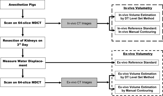
Eight Yorkshire breed anesthetized pigs (weight range 45–50 kg) were scanned on a 64-slice multidetector CT scanner (Sensation 64; Siemens) after injection of an iodinated (300 mg I/ml) contrast agent through an IV cannula. The kidneys of the pigs were then surgically resected and scanned by CT in the same manner. Both in vivo and ex vivo CT images were subjected to our computerized volumetry using DT level set method. The resulting volumes of the kidneys were compared with in vivo and ex vivo reference standards: the former was established by manual contouring of the kidneys on the CT images by an experienced radiologist, and the latter was established as the water displacement volume of the resected kidney.

Results

The comparisons of the in vivo and ex vivo measurements by our volumetric scheme with the associated reference standards yielded a mean difference of 1.73 ± 1.24% and 3.38 ± 2.51%, respectively. The correlation coefficients were 0.981 and 0.973 for in vivo and ex vivo comparisons, respectively. The mean difference between in vivo and ex vivo reference standards was 5.79 ± 4.26%, and the correlation coefficient between the two standards was 0.760.

Conclusion

Our computerized volumetry using the DT level set method can provide accurate in vivo and ex vivo measurements of kidney volume, despite a large difference between the two reference standards. This technique can be employed in human subjects for the determination of renal volume for preoperative surgical planning and assessment of oncology treatment.

Precise organ volumetry is gaining significance in various clinical settings for patient selection for an appropriate management, surgery planning, and monitoring a disease status ( ). Traditionally, kidney size/diameter measurement on imaging has been used as a surrogate to supplement these clinical needs. However, the kidney size measurement is an imperfect measure of overall organ volume. Three-dimensional kidney volumetry is more preferred in living kidney donors ( ), in assessing progression of polycystic renal disease ( ), and for tumor burden and treatment response evaluation ( ). With the recent introduction of MDCT scanners, there has been astronomical increase in the use of image postprocessing and three-dimensional services. Therefore, organ volumetry, although more desirable, is not routinely performed in lieu of the expertise required and substantial processing time. In addition, there is no known scientifically validated commercially available software that enables the organ volumetry in an automated fashion.

Segmentation of the kidney from CT images is an essential step for renal volumetry. However, manual segmentation of a kidney requires contouring of the kidney boundary on each renal CT image, which is labor intensive and prone to interoperator variability. Computerized volumetry (CV), on the other hand, relies on an efficient and accurate segmentation method, which is a subject of active research in medical image processing ( ). To reduce the labor of manual contouring, it is common to use a two-dimensional deformable model, i.e., a closed deformable curve, often called a snake ( ), to assist in user contouring. This model requires initialization of the curve on each axial image.

Get Radiology Tree app to read full this article<

Materials and methods

Study Design

Get Radiology Tree app to read full this article<

Dynamic-Threshold Level Set Method

Get Radiology Tree app to read full this article<

S={x|(x)=k}}, S

{

(

)

}

where k is an arbitrary scalar value (often zero, called zero-level set). Detailed descriptions of the level set method can be found in Refs. and .

Get Radiology Tree app to read full this article<

∙∙t=FDT(x)|∇|+CCurvature∇⋅(∇|∇|)|∇|+CSM∇2, •

•

(

)

∇

⋅

(

∇

)

∇

where C Curvature and C SM are two control parameters smoothing the segmentation results. In this study, C Curvature and C SM were empirically set to 0.5 and 0.2, respectively.

Get Radiology Tree app to read full this article<

Threshold shift

Get Radiology Tree app to read full this article<

Pf⋅Pf(Topt)=Pb⋅Pb(Topt), P

⋅

(

)

⋅

(

)

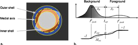
where P f and P b are the a priori probabilities of each material, which satisfy P f + P b = 1. P f and P b correspond to the percentages of the volume of each material in the images. P f and P b are the PDF functions of the foreground and background.

Get Radiology Tree app to read full this article<

Topt∣∣FtB<1>Topt|FtB=1(Ttheory)>Topt|FtB>1, T

(

)

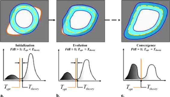
where FtB = v f /v b , which is the volumetric ratio of the foreground material to the background material in the histogram. In other words, the optimal threshold that separates two materials shifts toward the small region in a histogram relative to the theoretic threshold value. The threshold shift, T opt − T theory , is negative when v f > v b , whereas it is positive when v f < v b . Only when FtB = 1 ( v f = v b ), i.e., the histogram is balanced, is T opt equal to T theory .

Get Radiology Tree app to read full this article<

Dynamic-thresholding speed function

Get Radiology Tree app to read full this article<

FDT(x;Iopt)=sign(ΔI(x))⋅|ΔI(x)|n, F

(

;

)

(

)

⋅

(

)

where sign(x) is a sign function (also known as an indicator function), which is 1 if x is positive and −1 if x is negative; and n is often set to 2 or 3. ΔI(x) is defined by;

ΔI⎛⎝⎜⎜⎜⎜x⎞⎠⎟⎟⎟⎟=⎧⎩⎨⎪⎪⎪⎪⎪⎪⎪⎪−1(I(x)−Iopt)/ΔB(I(x)−Iopt)/ΔF1ifI(x)≤Iopt−ΔBifI(x)≤IoptifI(x)≤Iopt+ΔFifI(x)>Iopt+ΔF, Δ

(

)

{

−

(

)

≤

−

(

)

−

)

(

)

≤

(

)

−

)

(

)

≤

(

)

where Δ B and Δ F are the distance between the peak of the background in the histogram and the optimal threshold I opt , and the peak of foreground in the histogram to optimal threshold I opt , respectively ( Fig. 2 ).

Get Radiology Tree app to read full this article<

Results

Get Radiology Tree app to read full this article<

In Vivo and Ex Vivo Comparison

Get Radiology Tree app to read full this article<

Diff(VR,VX)=|VX−VR|VR⋅100%, D

(

)

−

⋅

100

where V R is the volume of the RS, and V X is the measured experimental volume. Six groups of comparison were performed, including the comparison between in vivo CV and in vivo RS, the comparison between ex vivo CV and ex vivo RS, the comparison between in vivo RS and ex vivo RS, the comparison between ex vivo RS and in vivo CV, the comparison between ex vivo RS and ex vivo manual volumetry (MV), and the comparison between ex vivo MV and ex vivo CV. We calculated the difference of the volume for each individual kidney in each comparison group. The statistical results are summarized in Table 1 .

Table 1

Statistical Results of Comparison Among In Vivo Reference Standard (RS), Ex Vivo RS, In Vivo Computerized Volumetry (CV), Ex Vivo CV, and Ex Vivo Manual Volumetry (MV)

Diff ( V R , V X ) Mean Difference (%) SD (%) Median Difference (%) Correlation Coefficient In vivo RS, in vivo CV 1.73 1.24 1.45 0.981 Ex vivo RS, ex vivo CV 3.36 2.54 2.75 0.972 In vivo RS, ex vivo RS 5.79 4.26 4.91 0.760 Ex vivo RS, in vivo CV 4.71 4.14 3.06 0.835 Ex vivo RS, ex vivo MV 14.77 2.20 15.19 0.913 Ex vivo MV, ex vivo CV 13.42 3.32 13.29 0.934

Get Radiology Tree app to read full this article<

Discussion

Get Radiology Tree app to read full this article<

Conclusion

Get Radiology Tree app to read full this article<

References

1. Yonemura Y., Taketomi A., Soejima Y., et. al.: Validity of preoperative volumetric analysis of congestion volume in living donor liver transplantation using three-dimensional computed tomography. Liver Transpl 2005; 11: pp. 1556-1562.
2. Dempsey M.F., Condon BR D.M.H.: Measurement of tumor “size” in recurrent malignant glioma: 1D, 2D, or 3D?. AJNR Am J Neuroradiol 2005; 26: pp. 770-776.
3. Herts B.: Role of three-dimensional imaging in surgical planning for kidney surgery. BJU Int 2005; 95: pp. 16-20.
4. Sise C., Kusaka M., Wetzel L.H., et. al.: Volumetric determination of progression in autosomal dominant polycystic kidney disease by computed tomography. Kidney Int 2000; 58: pp. 2492-2501.
5. Kim D., Park J.: Computer-aided detection of kidney tumor on abdominal computed tomography scans. Acta Radiol 2004; 45: pp. 791-795.
6. Ozono S., Miyao N., Igarashi T., et. al.: Tumor doubling time of renal cell carcinoma measured by CT: Collaboration of Japanese Society of Renal Cancer. Jpn J Clin Oncol 2004; 34: pp. 82-85.
7. Yoo T.S.: 2004.A K Peters, LtdWellesey
8. Sonka M., Fitzpatrick J.M.: 2004.SPIE−The International Society for Optical EngineeringBellingham
9. Kass M., Witkin A., Terzoopoulos D.: Snakes: active contour models. Int J Comput Vision 1988; 1: pp. 321-331.
10. Kim S., Yoo S., Kim S., Kim J., Park J.: Segmentation of kidney without using contrast medium on abdominal CT image.2000.pp. 1147-1152. In: 5th Int Conf Signal Processing. Beijing, China
11. Lin D., Lei C., Hung S.: Computer-aided kidney segmentation on abdominal CT images. IEEE Trans Inf Technol Biomed 2006; 10: pp. 59-65.
12. Pohle R., Toennies K.D.: Segmentation of medical images using adaptive region growing. Proc SPIE 2001; pp. 1337-1346.
13. Rao M., Stough J., Chi Y.Y., et. al.: Comparison of human and automatic segmentations of kidneys from CT images. Int J Radiat Oncol Biol Phys 2005; 61: pp. 954-960.
14. Tsagaan B., Shimizu A., Kobatake H., Miyakawa K.: An automated segmentation method of kidney using statistical information.2000.pp. 556-563. In: Proc Medical Image Computing and Computer Assisted Intervention
15. Wang X., He L., Wee W.: Deformable contour method: A constrained optimization approach. Int J Comput Vision 2004; 59: pp. 87-108.
16. Kobashi M., Shapiro L.: Knowledge-based organ identification from CT images. Pattern Recogn 1995; 28: pp. 475-491.
17. Brown M., Feng W., Hall T., et. al.: Knowledge-based segmentation of pediatric kidneys in CT for measurement of parenchymal volume. J Comput Assist Tomogr 2001; 25: pp. 639-648.
18. Osher S., Sethian J.: Fronts propagating with curvature-dependent speed: Algorithms based on Hamilton–Jacobi formulations. J Comput Phys 1988; 79: pp. 12-49.
19. Sethian J.: Level Set Methods: Evolving Interfaces in Geometry, Fluid Mechanics, Computer Vision and Material Sciences.1996.Cambridge University Press
20. Osher S., Fedkiw R.: 2002.Springer-VerlagNew York
21. Sean S., Bullitt E., Gerig G.: Level set evolution with region competition: automatic 3D segmentation of brain tumors.2002.pp. 532-535. In: International Conference on Pattern Recognition
22. Moss A.A., Friedman M.A., Brito A.C.: Determination of liver, kidney, and spleen volumes by computed tomography: An experimental study in dogs. J Comput Assist Tomogr 1981; 5: pp. 12-14.
23. Brenner D., Whitley N., Houk T., et. al.: Volume determinations in computed tomography. JAMA 1982; 247: pp. 1299-1302.
24. Kim J.: Animal study of renal volume measurement on abdominal CT using digital image processing: Preliminary report. Clin Imaging 2004; 28: pp. 135-137.
25. Cai W., Harris G., Yoshida H.: Computer-aided volumetrics of liver tumor in hepatic CT images.2006.pp. 375-377. In: Computed Assisted Radiology and Surgery. Osaka

Dynamic-Threshold Level Set Method for Volumetry of Porcine Kidney in CT Images

Rationale and Objective

Methods and Materials

Results

Conclusion

Materials and methods

Study Design

Dynamic-Threshold Level Set Method

Threshold shift

Dynamic-thresholding speed function

Results

In Vivo and Ex Vivo Comparison

Discussion

Conclusion

References

Further Reading

“Binary” and “Non-Binary” Detection Tasks Are Current Performance Measures Optimal?

2D or Not 2D That is the Question, But 3D is the Answer

3D and 2D Delayed-Enhancement Magnetic Resonance Imaging for Detection of Myocardial Infarction Preclinical and Clinical Results