
Rationale and Objectives
This study aimed to assess the effect of matrix size on the spatial resolution and image quality of ultra-high-resolution computed tomography (U-HRCT).
Materials and Methods
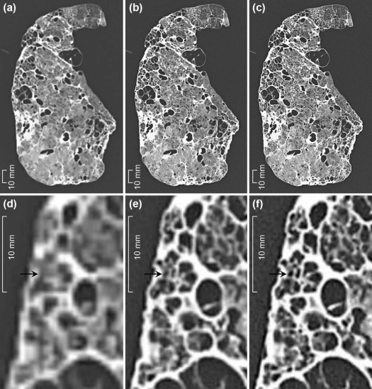
Slit phantoms and 11 cadaveric lungs were scanned on U-HRCT. Slit phantom scans were reconstructed using a 20-mm field of view (FOV) with 1024 matrix size and a 320-mm FOV with 512, 1024, and 2048 matrix sizes. Cadaveric lung scans were reconstructed using 512, 1024, and 2048 matrix sizes. Three observers subjectively scored the images on a three-point scale (1 = worst, 3 = best), in terms of overall image quality, noise, streak artifact, vessel, bronchi, and image findings. The median score of the three observers was evaluated by Wilcoxon signed-rank test with Bonferroni correction. Noise was measured quantitatively and evaluated with the Tukey test. A P value of <.05 was considered significant.
Results
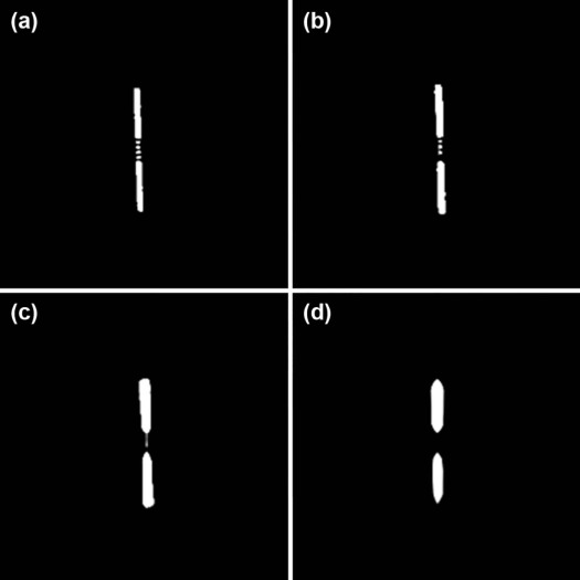
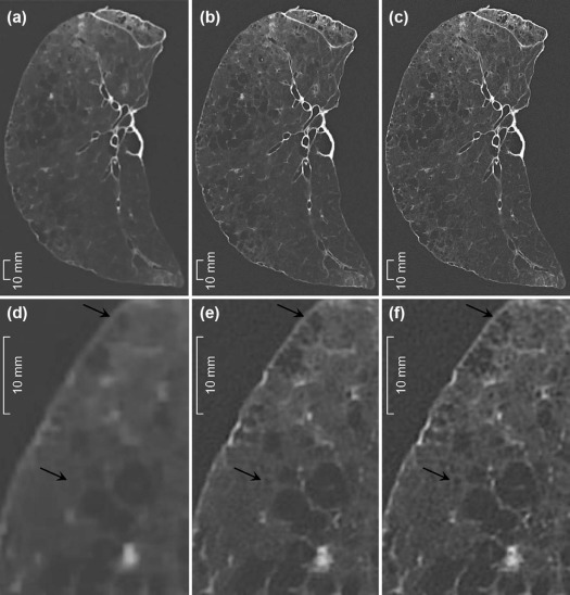
The maximum spatial resolution was 0.14 mm; among the 320-mm FOV images, the 2048 matrix had the highest resolution and was significantly better than the 1024 matrix in terms of overall quality, solid nodule, ground-glass opacity, emphysema, intralobular reticulation, honeycombing, and clarity of vessels ( P < .05). Both the 2048 and 1024 matrices performed significantly better than the 512 matrix ( P < .001), except for noise and streak artifact. The visual and quantitative noise decreased significantly in the order of 512, 1024, and 2048 ( P < .001).
Conclusion
In U-HRCT scans, a large matrix size maintained the spatial resolution and improved the image quality and assessment of lung diseases, despite an increase in image noise, when compared to a 512 matrix size.
Introduction
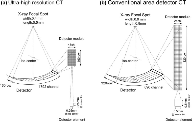
Advances in computed tomography (CT) have revolutionized diagnostic imaging. Various techniques, such as high-resolution CT, which was introduced in the 1980s, contributed to improvements in the spatial resolution of CT imaging . Recently, ultra-high-resolution CT (U-HRCT), which has smaller detector element and x-ray tube focus size than those of conventional CT, has become commercially available. Kakinuma et al. reported that a prototype U-HRCT provided better image quality of lung nodules than conventional CT . They also reported that the spatial resolution of the U-HRCT was 0.12 mm, whereas that of conventional CT ranged from 0.23 mm to 0.35 mm .
As for matrix size, 512 × 512 has been used in conventional CT, but larger matrix sizes, such as 1024 × 1024 and 2048 × 2048, are available with U-HRCT. When the reconstruction of the field of view (FOV) is set to 320 mm to cover the entire lung, the theoretical size of 1 pixel in an image matrix is 0.625 mm for 512 × 512; 0.313 mm for 1024 × 1024; and 0.156 mm for 2048 × 2048 ( Fig 1 ). Table 1 shows the theoretical size of 1 pixel according to matrix size and FOV reconstruction. We hypothesized that the size of 1 pixel in a smaller matrix image is much larger than the maximum spatial resolution of an U-HRCT scanner and insufficient to demonstrate the high spatial resolution of U-HRCT; on the other hand, a large matrix size may maintain the spatial resolution and improve the image quality of lung CT.
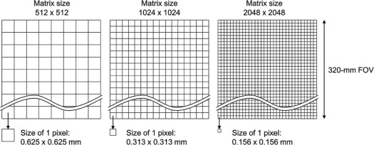
TABLE 1
The Theoretical Sizes of 1 Pixel According to Matrix Size and Reconstruction FOV
Reconstruction FOV 400 mm 320 mm 300 mm 200 mm 100 mm 75 mm Matrix size 512 × 512 0.781 0.625 0.586 0.391 0.195 0.146 1024 × 1024 0.391 0.313 0.293 0.195 0.098 0.073 2048 × 2048 0.195 0.156 0.146 0.098 0.049 0.036
FOV, field of view.
The unit of the theoretical sizes of 1 pixel is mm.
Get Radiology Tree app to read full this article<
Get Radiology Tree app to read full this article<
Materials and Methods
U-HRCT Scanner
Get Radiology Tree app to read full this article<
Get Radiology Tree app to read full this article<
Slit Phantom Evaluation
Get Radiology Tree app to read full this article<
Cadaveric Lung and Image Acquisition
Get Radiology Tree app to read full this article<
Get Radiology Tree app to read full this article<
Subjective Image Analysis
Get Radiology Tree app to read full this article<
Get Radiology Tree app to read full this article<
Objective Noise Analysis
Get Radiology Tree app to read full this article<
Statistical Analysis
Get Radiology Tree app to read full this article<
Results
Slit Phantom Evaluation
Get Radiology Tree app to read full this article<
Get Radiology Tree app to read full this article<
Subjective Image Analysis of Cadaveric Lungs
Get Radiology Tree app to read full this article<
TABLE 2
Comparison of the Subjective Analysis Scores Among the Matrix Sizes
N Score (Mean ± SD)P Value 2048 1024 512 2048 vs 1024 2048 vs 512 1024 vs 512 Overall image quality 33 2.8 ± 0.4 2.0 ± 0.0 1.0 ± 0.0 <.001 \* <.001 \* <.001 \* Noise 33 1.0 ± 0.0 2.0 ± 0.0 3.0 ± 0.0 <.001 \* <.001 \* <.001 \* Streak artifact 33 2.0 ± 0.2 2.0 ± 0.2 2.0 ± 0.2 1 1 1 Clarity of small vessel 29 2.2 ± 0.4 2.0 ± 0.0 1.0 ± 0.0 .014 \* <.001 \* <.001 \* Clarity of small bronchi 29 2.1 ± 0.4 2.0 ± 0.0 1.0 ± 0.0 .046 <.001 \* <.001 \* Solid nodule 26 2.4 ± 0.5 2.0 ± 0.0 1.0 ± 0.0 .002 \* <.001 \* <.001 \* Faint nodule 11 2.4 ± 0.5 2.0 ± 0.0 1.0 ± 0.0 .046 .002 \* .001 \* Ground-glass opacity 25 2.3 ± 0.5 2.0 ± 0.0 1.0 ± 0.0 .008 \* .002 \* .001 \* Consolidation 11 2.2 ± 0.4 2.0 ± 0.0 1.0 ± 0.0 .157 .002 \* .001 \* Emphysema 12 2.6 ± 0.5 2.0 ± 0.0 1.0 ± 0.0 .008 \* .002 \* .001 \* Interlobular septal thickening 15 2.3 ± 0.5 1.9 ± 0.3 1.1 ± 0.2 .059 .001 \* <.001 \* Bronchovascular bundle thickening 12 2.0 ± 0.0 2.0 ± 0.0 1.0 ± 0.0 1 .001 \* .001 \* Intralobular reticulation 12 2.5 ± 0.5 2.0 ± 0.0 1.0 ± 0.0 .014 \* .002 \* .001 \* Bronchiectasis 9 2.0 ± 0.0 1.9 ± 0.3 1.0 ± 0.0 .317 .003 \* .005 \* Honeycombing 11 2.9 ± 0.3 2.0 ± 0.0 1.0 ± 0.0 .002 \* .001 \* .001 \*
CT, computed tomography; N, the number of the evaluated areas for each CT finding; SD, standard deviation.
Get Radiology Tree app to read full this article<
Get Radiology Tree app to read full this article<
Get Radiology Tree app to read full this article<
Get Radiology Tree app to read full this article<
Objective Image Analysis
Get Radiology Tree app to read full this article<
Discussion
Get Radiology Tree app to read full this article<
Get Radiology Tree app to read full this article<
Get Radiology Tree app to read full this article<
Get Radiology Tree app to read full this article<
Get Radiology Tree app to read full this article<
Get Radiology Tree app to read full this article<
Get Radiology Tree app to read full this article<
Get Radiology Tree app to read full this article<
Acknowledgments
Get Radiology Tree app to read full this article<
References
1. Todo G., Ito H., Nakano Y., et. al.: High resolution CT (HR-CT) for the evaluation of pulmonary peripheral disorders. Rinsho Hoshasen 1982; 27: pp. 1319-1326.
2. Kakinuma R., Moriyama N., Muramatsu Y., et. al.: Ultra-high-resolution computed tomography of the lung: image quality of a prototype scanner. PLoS ONE 2015; 10: pp. e0137165.
3. Yanagawa M., Tomiyama N., Honda O., et. al.: Multidetector CT of the lung: image quality with garnet-based detectors. Radiology 2010; 255: pp. 944-954.
4. Tsukagoshi S., Ota T., Fujii M., et. al.: Improvement of spatial resolution in the longitudinal direction for isotropic imaging in helical CT. Phys Med Biol 2007; 52: pp. 791-801.
5. Markarian B., Dailey E.T.: Preparation of inflated lung specimens.Groskin S.A.Heitzman’s the lung: radiologic-pathologic correlations.1993.MosbySt. Louis:pp. 4-12.
6. Boehm T., Willmann J.K., Hilfiker P.R., et. al.: Thin-section CT of the lung: does electrocardiographic triggering influence diagnosis?. Radiology 2003; 229: pp. 483-491.
7. Zhu H., Zhang L., Wang Y., et. al.: Improved image quality and diagnostic potential using ultra-high-resolution computed tomography of the lung with small scan FOV: a prospective study. PLoS ONE 2017; 12: pp. 1-11.
8. Mayo J.R., Webb W.R., Gould R., et. al.: High-resolution CT of the lungs: an optimal approach. Radiology 1987; 163: pp. 507-510.
9. Murata K., Khan A., Rojas K.A., et. al.: Optimization of computed tomography technique to demonstrate the fine structure of the lung. Invest Radiol 1988; 23: pp. 170-175.
10. Yanagawa M., Gyobu T., Leung A.N., et. al.: Ultra-low-dose CT of the lung: effect of iterative reconstruction techniques on image quality. Acad Radiol 2014; 21: pp. 695-703.
11. Pickhardt P.J., Lubner M.G., Kim D.H., et. al.: Abdominal CT with model-based iterative reconstruction (MBIR): initial results of a prospective trial comparing ultralow-dose with standard-dose imaging. AJR Am J Roentgenol 2012; 199: pp. 1266-1274.