
Rationale and Objectives
Tissue perfusion is commonly used to evaluate lung tumor lesions through dynamic contrast-enhanced computed tomography (DCE-CT). The aim of this study was to improve the reliability of the blood flow (BF) maps by means of a guided sampling of the tissue time–concentration curves (TCCs).
Materials and Methods
Fourteen selected CT perfusion (CTp) examinations from different patients with lung lesions were considered, according to different degrees of motion compensation. For each examination, two regions of interest (ROIs) referring to the target lesion and the arterial input were manually segmented. To obtain the perfusion parameters, we computed the maximum slope of the Hill equation, describing the pharmacokinetics of the contrast agent, and the TCC was fitted for each voxel. A guided iterative approach based on the Random Sample Consensus method was used to detect and exclude samples arising from motion artifacts through the assessment of the confidence level of each single temporal sample of the TCC compared to the model. Removing these samples permits to refine the model fitting, thus exploiting more reliable data. Goodness-of-fit measures of the fitted TCCs to the original data (eg, root mean square error and correlation distance) were used to assess the reliability of the BF values, so as to preserve the functional structure of the resulting perfusion map. We devised a quantitative index, the local coefficient of variation (lCV), to measure the spatial coherence of perfusion maps, from local to regional and global resolution. The effectiveness of the algorithm was tested under three different degrees of motion yielded by as many alignment procedures.
Results
At pixel level, the proposed approach improved the reliability of BF values, quantitatively assessed through the correlation index. At ROI level, a comparative analysis emphasized how our approach “replaced” the noisy pixels, providing smoother parametric maps while preserving the main functional structure. Moreover, the implemented algorithm provides a more meaningful effect in correspondence of a higher motion degree. This was confirmed both quantitatively, using the lCV, and qualitatively, through visual inspection by expert radiologists.
Conclusions
Perfusion maps achieved with the proposed approach can now be used as a valid tool supporting radiologists in DCE-CTp studies. This represents a step forward to clinical utilization of these studies for staging, prognosis, and monitoring values of therapeutic regimens.
Recently, dynamic contrast-enhanced computed tomography (DCE-CT) has become a major imaging technique in lung perfusion studies because by providing a high spatial and temporal resolution, it is particularly suitable for lung imaging . In fact, it is able to generate estimates of tissue perfusion that are useful for characterization and monitoring of the tumor’s lesion.
The functional and morphologic evaluation that can be achieved on the perfusion examinations has been proven to be effective to assist the diagnosis process , for therapy decision , and for patient monitoring . However, for a reliable quantification of tumor perfusion at voxel level, the technique still requires to be improved, and it is currently a matter of a number of studies .
Get Radiology Tree app to read full this article<
Get Radiology Tree app to read full this article<
Get Radiology Tree app to read full this article<
Get Radiology Tree app to read full this article<
Materials and methods
Patients and Protocols
Get Radiology Tree app to read full this article<
Table 1
Table Summarizing the Main Features of the Fourteen Tumor Lesions
Patient Lesion Type ID1 1 Adenocarcinoma, IV stadium ID2 1 Squamocellular carcinoma G2, IIIB stadium ID3 1 Adenocarcinoma, III stadium ID4 1 Adenocarcinoma, IV stadium ID5 1 Squamocellular carcinoma, G3 ID6 1 Adenocarcinoma, IV stadium ID7 1 Adenocarcinoma, (n.a.) ID8 1 Squamocellular carcinoma, G2-3, IB stadium ID9 1 Adenocarcinoma, (n.a.) ID10 1 Colloid adenocarcinoma, IV stadium ID11 1 Colloid adenocarcinoma, IV stadium ID12 1 EGFR adenocarcinoma, (n.a.) ID13 1 EGFR adenocarcinoma, (n.a.) ID14 1 EGFR adenocarcinoma, IV stadium
EGFR, epidermal growth factor receptor; n.a., not available.
Get Radiology Tree app to read full this article<
Get Radiology Tree app to read full this article<
Get Radiology Tree app to read full this article<
Image Registration
Get Radiology Tree app to read full this article<
Standard Fixed Mode (SM)
Get Radiology Tree app to read full this article<
Transverse Manual Registration (2D)
Get Radiology Tree app to read full this article<
Multislice Manual Registration (3D)
Get Radiology Tree app to read full this article<
Get Radiology Tree app to read full this article<
Perfusion Model
Get Radiology Tree app to read full this article<
Get Radiology Tree app to read full this article<
Get Radiology Tree app to read full this article<
yˆ(t)=E0+(EMAX−E0)tα(EC50)α+tα y
ˆ
(
t
)
=
E
0
+
(
E
MAX
−
E
0
)
t
α
(
E
C
50
)
α
+
t
α
where EC 50 is the instant of half-maximum response concentration of the curve and α is the nonlinear parameter mostly affecting the slope of the curve. The BF perfusion values are computed on pixel basis by applying the maximum slope method, whose details are given in Appendix B . Although, commonly in literature, the Hill equation is used in pharmacodynamic models to describe nonlinear drug dose–response relationships, it is also suited to model the pharmacokinetics of a contrast agent, and in particular the fraction of radioactivity in plasma . In such a way, the computation of perfusion is strengthened by the inclusion of a larger number of data points and, differently from the linear model , it allows preserving the actual trend of the TCCs, finally improving both robustness and accuracy.
Get Radiology Tree app to read full this article<
Get Radiology Tree app to read full this article<
Fitting Procedure
Get Radiology Tree app to read full this article<
Outlier Removal: Our Algorithm
Get Radiology Tree app to read full this article<
Get Radiology Tree app to read full this article<
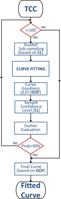
Get Radiology Tree app to read full this article<
Get Radiology Tree app to read full this article<
Colorimetric BF Map
Get Radiology Tree app to read full this article<
Validation
Get Radiology Tree app to read full this article<
Get Radiology Tree app to read full this article<
Get Radiology Tree app to read full this article<
Statistics
Get Radiology Tree app to read full this article<
Results
Get Radiology Tree app to read full this article<
Curve Fitting
Get Radiology Tree app to read full this article<
Get Radiology Tree app to read full this article<
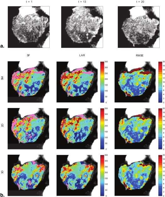
Image Registration
Get Radiology Tree app to read full this article<
Table 2
Replaced Pixels for Each Alignment Procedure and Values Referring to 3D Alignment, for the Considered Lesions
Area (Pixel) Percent Replaced 3D 3D 2D SM Fitting BF (μ ± σ) RMSE (μ) CD (μ) gCV lCV (μ ± σ) ID1 3385 14.06 18.26 19.47 SF 82.98 ± 55.97 7.80 0.269 0.713 0.602 ± 0.098 LAR 88.36 ± 53.95 7.87 0.181 0.611 0.538 ± 0.089 ID2 4405 23.16 24.34 23.68 SF 135.39 ± 63.5 9.09 0.212 0.498 0.412 ± 0.225 LAR 141.83 ± 64.73 9.28 0.145 0.456 0.390 ± 0.203 ID3 1559 7.25 11.03 16.10 SF 59.19 ± 26.12 11.10 0.224 0.519 0.375 ± 0.074 LAR 60.23 ± 26.46 11.18 0.179 0.439 0.368 ± 0.069 ID4 4732 9.38 14.69 13.33 SF 131.15 ± 77.30 9.72 0.268 0.660 0.540 ± 0.084 LAR 134.28 ± 74.46 9.84 0.170 0.555 0.499 ± 0.072 ID5 926 9.07 13.17 13.27 SF 51.45 ± 36.70 6.95 0.052 0.800 0.515 ± 0.138 LAR 53.62 ± 37.16 6.96 0.041 0.693 0.489 ± 0.136 ID6 1833 9.49 13.42 15.60 SF 67.00 ± 44.43 8.82 0.251 0.765 0.623 ± 0.114 LAR 69.95 ± 42.94 8.89 0.198 0.614 0.573 ± 0.095 ID7 3709 15.10 15.72 17.44 SF 100.35 ± 41.42 10.89 0.226 0.418 0.374 ± 0.129 LAR 104.41 ± 38.98 10.97 0.174 0.373 0.329 ± 0.111 ID8 477 7.13 10.90 20.13 SF 106.77 ± 43.08 7.87 0.066 0.476 0.393 ± 0.145 LAR 106.00 ± 41.65 7.95 0.062 0.393 0.380 ± 0.145 ID9 671 13.41 14.46 17.29 SF 47.83 ± 30.89 13.39 0.243 0.905 0.570 ± 0.186 LAR 47.32 ± 28.94 13.87 0.231 0.612 0.558 ± 0.182 ID10 550 13.36 25.09 26.36 SF 79.76 ± 42.03 22.42 0.304 0.591 0.493 ± 0.089 LAR 79.51 ± 40.82 22.56 0.212 0.513 0.484 ± 0.081 ID11 470 13.19 19.57 12.98 SF 53.19 ± 33.74 10.57 0.360 0.661 0.604 ± 0.066 LAR 55.41 ± 35.57 10.65 0.348 0.642 0.605 ± 0.066 ID12 726 26.86 27.01 24.38 SF 75.45 ± 86.65 8.94 0.253 1.353 1.135 ± 0.140 LAR 77.27 ± 81.52 9.29 0.201 1.055 1.029 ± 0.099 ID13 927 26.97 22.11 27.83 SF 22.28 ± 20.84 6.70 0.267 1.446 0.933 ± 0.131 LAR 25.03 ± 20.44 6.76 0.248 0.817 0.817 ± 0.101 ID14 2492 12.04 12.80 14.49 SF 61.45 ± 46.10 6.50 0.251 0.822 0.627 ± 0.163 LAR 62.26 ± 44.68 6.55 0.216 0.718 0.595 ± 0.151
BF, blood flow; CD, correlation distance; gCV, global coefficient of variation; LAR, Look And Replace; lCV, local coefficient of variation; RMSE, root mean square error; SF, Standard Fitting; SM, standard fixed mode.
From left to right: lesion ID, lesion’s extent (in pixels), percentage of pixels replaced by the Look And Replace algorithm, and for each fitting procedure used, the associated blood flow (mean and standard deviation), mean root mean square error and correlation distance, and the global coefficient of variation along with the local coefficient of variation computed over 7 × 7 windows (mean and standard deviation).
Get Radiology Tree app to read full this article<
Get Radiology Tree app to read full this article<
Get Radiology Tree app to read full this article<
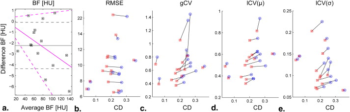
Functional and Structural Coherence
Get Radiology Tree app to read full this article<
Get Radiology Tree app to read full this article<
Get Radiology Tree app to read full this article<
Get Radiology Tree app to read full this article<
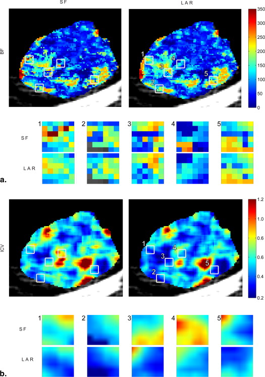
Table 3
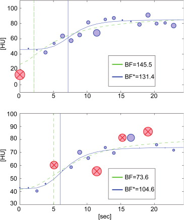
Values Referring to the Regions Shown in Figure 5 , and Obtained by the Standard Fitting and Look And Replace Algorithms
Fitting BF (μ ± σ) RMSE (μ) CD (μ) lCV R1 SF 161.90 ± 80.46 7.28 0.077 0.497 LAR 154.78 ± 55.78 7.44 0.078 0.360 R2 SF 141.53 ± 64.21 8.15 0.074 0.454 LAR 151.91 ± 53.62 8.27 0.073 0.353 R3 SF 176.17 ± 62.06 7.70 0.139 0.352 LAR 177.19 ± 53.20 7.75 0.137 0.300 R4 SF 86.32 ± 73.61 7.83 0.250 0.853 LAR 87.01 ± 44.44 7.96 0.246 0.511 R5 SF 127.51 ± 77.52 9.81 0.219 0.608 LAR 147.86 ± 56.12 10.10 0.216 0.380
BF, blood flow; CD, correlation distance; LAR, Look And Replace; lCV, local coefficient of variation; RMSE, root mean square error; SF, Standard Fitting.
Blood Flow (Mean and Standard Deviation), Root Mean Square Error (Mean), Correlation Distance (Mean), and Local Coefficient of Variation Computed Over the 5 couples of Regions.
Get Radiology Tree app to read full this article<
Get Radiology Tree app to read full this article<
Get Radiology Tree app to read full this article<
Discussion
Get Radiology Tree app to read full this article<
Get Radiology Tree app to read full this article<
Get Radiology Tree app to read full this article<
Get Radiology Tree app to read full this article<
Get Radiology Tree app to read full this article<
Get Radiology Tree app to read full this article<
Acknowledgments
Get Radiology Tree app to read full this article<
Appendix A
Formulas of RMSE and CD
Get Radiology Tree app to read full this article<
RMSE=∑Nt=1(yt−ŷt)2n−−−−−−−−−√ R
M
S
E
=
∑
t
=
1
N
(
y
t
−
ŷ
t
)
2
n
whereas the CD index is computed through Equation A.2 :
CD=⎛⎝1−Cov(yt,ŷt)σytσŷt2⎞⎠ C
D
=
(
1
−
Cov
(
y
t
,
ŷ
t
)
σ
y
t
σ
ŷ
t
2
)
where N is the number of time samples, y ( t ) the sample concentration, and ŷ ( t ) the values of the fitted curve. The Cov operator computes the covariance between the y__t and ŷ__t signals.
Get Radiology Tree app to read full this article<
Appendix B
Maximum slope computation
Get Radiology Tree app to read full this article<
BF=dŷ(t)dt∣∣maxa(t)|max B
F
=
d
ŷ
(
t
)
d
t
|
m
a
x
a
(
t
)
|
m
a
x
Get Radiology Tree app to read full this article<
Get Radiology Tree app to read full this article<
References
1. Li Y., Yang Z.G., Chen T.W., et. al.: Whole tumour perfusion of peripheral lung carcinoma: evaluation with first-pass CT perfusion imaging at 64-detector row CT. Clin Radiol 2008; 63: pp. 629-635.
2. Chen B., Barnhart H., Richard S., et. al.: Quantitative CT: technique dependence of volume estimation on pulmonary nodules. Phys Med Biol 2012; 57: pp. 1335-1348.
3. Sauter A.W., Merkle A., Schulze M., et. al.: Intraobserver and interobserver agreement of volume perfusion CT (VPCT) measurements in patients with lung lesions. Eur J Radiol 2012; 81: pp. 2853-2859.
4. Sluimer I., Schilham A., Prokop M., et. al.: Computer analysis of computed tomography scans of the lung: a survey. Medical Imaging, IEEE Transactions on 2006; 25: pp. 385-405.
5. Sitartchouk I., Roberts H., Pereira A., et. al.: Computed tomography perfusion using first pass methods for lung nodule characterization. Investigative Radiology 2008; 40: pp. 052502.
6. Ng Q.S., Goh V.: Angiogenesis in non-small cell lung cancer: imaging with perfusion computed tomography. J Thorac Imaging 2010; 25: pp. 142-150.
7. Miles K.A., Griffiths M.R., Keith C.J.: Blood flow-metabolic relationships are dependent on tumour size in non-small cell lung cancer: a study using quantitative contrast-enhanced computer tomography and positron emission tomography. Eur. J. Nucl. Med. Mol. Imaging 2006; 33: pp. 22-28.
8. Lind J.S., Meijerink M.R., Dingemans A.M., et. al.: Dynamic contrast-enhanced CT in patients treated with sorafenib and erlotinib for non-small cell lung cancer: a new method of monitoring treatment?. Eur Radiol 2010; 20: pp. 2890-2898.
9. Ganeshan B., Miles K.A.: Quantifying tumour heterogeneity with CT. Cancer imaging 2013; 13: pp. 140-149.
10. Koh T.S., Shi W., Thng C.H., et. al.: Assessment of tumor blood flow distribution by dynamic contrast-enhanced CT. IEEE Trans Med Imaging 2013; 32: pp. 1504-1514.
11. Shan F., Xing W., Qiu J., et. al.: First-pass CT perfusion in small peripheral lung cancers: effect of the temporal interval between scan acquisitions on the radiation dose and quantitative vascular parameters. Academic radiology 2013; 20: pp. 972-979.
12. Yeung T., Dekaban M., De Haan N., et. al.: Improving quantitative CT perfusion parameter measurements using principal component analysis. Academic Radiology 2014; 21: pp. 624-632.
13. Miles K., Hayball M., Dixon A.: Colour perfusion imaging: a new application of computed tomography. The Lancet 1991; 337: pp. 643-645.
14. Brix G., Zwick S., Griebel J., et. al.: Estimation of tissue perfusion by dynamic contrast-enhanced imaging: simulation-based evaluation of the steepest slope method. Eur Radiol 2010; 20: pp. 2166-2175.
15. Chandler A., Wei W., Herron D., et. al.: Semiautomated motion correction of tumors in lung CT-perfusion studies. Academic radiology 2011; 18: pp. 286-293.
16. Fischler M.A., Bolles R.C.: Random sample consensus: a paradigm for model fitting with applications to image analysis and automated cartography. Commun. ACM 1981; 24: pp. 381-395.
17. Raguram R., Chum O., Pollefeys M., et. al.: USAC: a universal framework for random sample consensus. Pattern Analysis and Machine Intelligence, IEEE Transactions on 2013; 35: pp. 2022-2038.
18. Torr P.H., Zisserman A.: MLESAC: a new robust estimator with application to estimating image geometry. Computer Vision and Image Understanding 2000; 78: pp. 138-156.
19. Tordoff B.J., Murray D.W.: Guided-MLESAC: faster image transform estimation by using matching priors. IEEE Trans Pattern Anal Mach Intell 2005; 27: pp. 1523-1535.
20. Chum O, Matas J, Matching with PROSAC-progressive sample consensus, In: IEEE Computer Society Conference on Computer Vision and Pattern Recognitio (CVPR), 2005. Vol. 1, IEEE, 2005, pp. 220–226.
21. Kang M., Gao J., Tang L.: Nonlinear RANSAC optimization for parameter estimation with applications to phagocyte transmigration. Proc Int Conf Mach Learn Appl 2011; 1: pp. 501-504.
22. Wang M.H., Palmeri M.L., Rotemberg V.M., et. al.: Improving the robustness of time-of-flight based shear wave speed reconstruction methods using RANSAC in human liver in vivo. Ultrasound Med Biol 2010; 36: pp. 802-813.
23. You W., Simalatsar A., De Micheli G.: Parameterized SVM for personalized drug concentration prediction. Conf Proc IEEE Eng Med Biol Soc 2013; 2013: pp. 5789-5792.
24. Mullani N., Gould K.: First-pass measurements of regional blood flow with external detectors. Journal of nuclear medicine: official publication, Society of Nuclear Medicine 1983; 24: pp. 577-581.
25. Li K., Zhu X., Checkley D., et. al.: Simultaneous mapping of blood volume and endothelial permeability surface area product in gliomas using iterative analysis of first-pass dynamic contrast enhanced MRI data. Br J Radiol 2003; 76: pp. 39-50.
26. Naish J., McGrath D., Bains L., et. al.: Comparison of dynamic contrast-enhanced MRI and dynamic contrast-enhanced CT biomarkers in bladder cancer. Magnetic Resonance in Medicine 2011; 66: pp. 219-226.
27. Vaupel P., Kallinowski F., Okunieff P.: Blood flow, oxygen and nutrient supply, and metabolic microenvironment of human tumors: a review. Cancer research 1989; 49: pp. 6449-6465.
28. Tsushima Y., Funabasama S., Sanada S., et. al.: Development of perfusion CT software for personal computers. Acad Radiol 2002; 9: pp. 922-926.
29. Reiner C.S., Goetti R., Burger I.A., et. al.: Liver perfusion imaging in patients with primary and metastatic liver malignancy: prospective comparison between 99mTc-MAA spect and dynamic CT perfusion. Acad Radiol 2012; 19: pp. 613-621.
30. Winterdahl M., Sorensen M., Keiding S., et. al.: Hepatic blood perfusion estimated by dynamic contrast-enhanced computed tomography in pigs: limitations of the slope method. Invest Radiol 2012; 47: pp. 588-595.
31. Miles K., Lee T., Goh V., et. al.: Current status and guidelines for the assessment of tumour vascular support with dynamic contrast-enhanced computed tomography. European radiology 2012; 22: pp. 1430-1441.
32. Harpen M.D., Lecklitner M.L.: Derivation of gamma variate indicator dilution function from simple convective dispersion model of blood flow. Med Phys 1984; 11: pp. 690-692.
33. Chan A., Nelson S.: Simplified gamma-variate fitting of perfusion curves.Biomedical imaging: nano to macro, 2004. IEEE International Symposium on.2004.pp. 1067-1070.
34. Neukirchen C, Rose G, Parameter estimation in a model based approach for tomographic perfusion measurement, In: Nuclear Science Symposium Conference Record, 2005 IEEE, Vol. 4, 2005, pp. 2235–2239.
35. Goutelle S., Maurin M., Rougier F., et. al.: The Hill equation: a review of its capabilities in pharmacological modelling. Fundam Clin Pharmacol 2008; 22: pp. 633-648.
36. Wu S., Ogden R., Mann J., et. al.: Optimal metabolite curve fitting for kinetic modeling of 11C-WAY-100635. Journal of Nuclear Medicine 2007; 48: pp. 926-931.
37. Jensen N.K., Lock M., Fisher B., et. al.: Prediction and reduction of motion artifacts in free-breathing dynamic contrast enhanced CT perfusion imaging of primary and metastatic intrahepatic tumors. Acad Radiol 2013; 20: pp. 414-422.
38. Hahn G., Meeker W.: Statistical intervals: a guide for practitioners2011.John Wiley & Sons
39. Zar J.: Biostatistical analysis.5th ed.2010.Pearson Prentice-HallUpper Saddle River, New Jersey
40. Benner T., Heiland S., Erb G., et. al.: Accuracy of gamma-variate fits to concentration-time curves from dynamic susceptibility-contrast enhanced MRI: influence of time resolution, maximal signal drop and signal-to-noise. Magnetic resonance imaging 1997; 15: pp. 307-317.
41. Ahearn T., Staff R., Redpath T., et. al.: The use of the Levenberg-Marquardt curve-fitting algorithm in pharmacokinetic modelling of DCE-MRI data. Phys. Med. Biol 2005; 50: pp. 307-317.
42. Ramirez-Villegas J., Ramirez-Moreno D.: Microcalcification detection in digitized mammograms: a neurobiologically-inspired approach.Stanciu S.G.Digital image processing.2011.InTechRijeka, Croatia:pp. 161-186.
43. Balvay D., Troprès I., Billet R., et. al.: Mapping the zonal organization of tumor perfusion and permeability in a rat glioma model by using dynamic contrast-enhanced synchrotron radiation CT. Radiology 2009; 250: pp. 692-702.