Estimating the Receiver Operating Characteristic Curve in Studies That Match Controls to Cases on Covariates

Rationale and Objectives

Studies evaluating a new diagnostic imaging test may select control subjects without disease who are similar to case subjects with disease in regard to factors potentially related to the imaging result. Selecting one or more controls that are matched to each case on factors such as age, comorbidities, or study site improves study validity by eliminating potential biases due to differential characteristics of readings for cases versus controls. However, it is not widely appreciated that valid analysis requires that the receiver operating characteristic (ROC) curve be adjusted for covariates. We propose a new computationally simple method for estimating the covariate-adjusted ROC curve that is appropriate in matched case-control studies.

Materials and Methods

We provide theoretical arguments for the validity of the estimator and demonstrate its application to data. We compare the statistical properties of the estimator with those of a previously proposed estimator of the covariate-adjusted ROC curve. We demonstrate an application of the estimator to data derived from a study of emergency medical services encounters where the goal is to diagnose critical illness in nontrauma, non–cardiac arrest patients. A novel bootstrap method is proposed for calculating confidence intervals.

Results

The new estimator is computationally very simple, yet we show it yields values that approximate the existing, more complicated estimator in simulated data sets. We found that the new estimator has excellent statistical properties, with bias and efficiency comparable with the existing method.

Conclusions

In matched case-control studies, the ROC curve should be adjusted for matching covariates and can be estimated with the new computationally simple approach.

Many factors can influence the assessment provided by a radiologist reading a diagnostic image . Patient characteristics, for example breast density in reading mammograms, are one source of variability. Characteristics of the radiologist including expertise, training and malpractice concerns can influence assessments . Interpretations vary with institutions and they vary with health care norms that change over time .

In research concerning the accuracy of diagnostic tests such factors are called covariates and they must be taken into account in study design and analysis. Consider for example a study to evaluate the accuracy of computer-assisted mammography (CAD-mammography) in detecting breast cancer. Since breast cancer is more common in older women, a random set of breast cancer cases is likely to be older than a random set of controls without breast cancer. Therefore, if controls are selected at random from the population of women who undergo mammography, differences in CAD-mammography assessments between cases and controls may be partly attributed to differences in their ages. In particular, a higher number of findings by CAD-mammography in cases may be partly due to the fact that it discovers anomalies more easily in fatty breast tissue that is more common in older women. Ignoring the covariate “age” that influences CAD-mammography assessments would lead to biased research results.

Get Radiology Tree app to read full this article<

Materials and methods

The Covariate-Adjusted ROC Curve

Get Radiology Tree app to read full this article<

ROCx(f)=Prob[Y>yx(f)|D=1,X=x] ROC

(

)

Prob

[

(

)

]

where f=Prob[Y>yx(f)|D=0,X=x] f

Prob

[

(

)

] . The covariate-adjusted ROC curve, denoted by A ROC, is the average covariate-specific ROC curve where the averaging is made with respect to the distribution of the cases across covariate levels:

AROC(f)=E{ROCx(f)}. A

ROC

(

)

{

ROC

(

)

}

Get Radiology Tree app to read full this article<

Existing Estimator of the AROC: The pv -AROC Estimator

Get Radiology Tree app to read full this article<

{(Di=1,Xi,Yi)i=1,…,n;(Dj=0,Xj,Yj)j=1,…,K×n} {

(

)

…

;

(

)

…

}

Get Radiology Tree app to read full this article<

Prob(Y<r|D,X)=Φ({θr−α1D−α2X}exp{β1D}) P

(

)

(

{

−

}

{

}

)

can be fit to the data, where Φ Φ is the standard normal cumulative distribution function . The A ROC is then calculated from the estimated model parameters:

AROC(f)=Φ(α1+Φ−1(f)exp{β1}), A

(

)

(

−1

(

)

exp

{

}

)

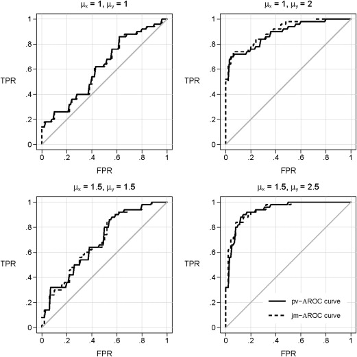
where f is the false positive rate. The second approach models the diagnostic test in controls only, using a semiparametric method. This model provides covariate-specific reference distributions for the test results with respect to which test results from cases are standardized . The A ROC is then calculated nonparametrically from the standardized values of the test results among cases . Although the two approaches are related, the second approach is more general and requires fewer assumptions. We focus on it here, call it the percentile value method, and use pv - A ROC to denote the resulting estimator of the A ROC. For a thorough discussion of the relationships between the percentile value method and the parametric modeling method, see References and .

Get Radiology Tree app to read full this article<

A New Method for Matched Data: The jm -AROC Estimator

Get Radiology Tree app to read full this article<

(i) Get Radiology Tree app to read full this article<

logitP(D=1|X,Y)=a0+a1×X+a2×Y+a3×X×Y logit

(

)

to the matched data set, but alternative forms for the risk model could be used such as a model without interaction terms that we will consider later. Note here that the matching covariates are included as predictors in the risk model. Get Radiology Tree app to read full this article<

(ii) Get Radiology Tree app to read full this article<

Get Radiology Tree app to read full this article<

Rationale for the jm -AROC Estimator

Get Radiology Tree app to read full this article<

Result

Get Radiology Tree app to read full this article<

TheROCcurveforthejointriskscores,P(D=1|X,Y),isthesameasthecovariate-adjustedROCcurve; The

ROC

curve

for

the

joint

risk

scores,

(

)

the

same

the

covariate-adjusted

ROC

curve;

if and only if

P(D=1|X)=P(D=1); P

(

)

(

)

;

[Note that the result as written in the Kerr and Pepe report uses somewhat different notation and has a small typo in the first item where ROCX|Y ROC

Y should be ROCY|X ROC

X .]

Get Radiology Tree app to read full this article<

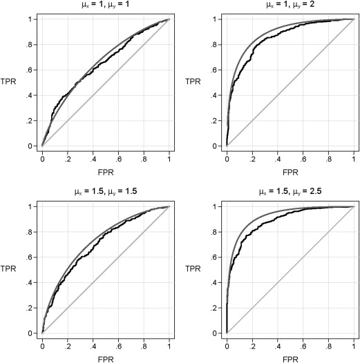
Data and Estimation Details for Simulation Studies

Get Radiology Tree app to read full this article<

AROC(f)=Φ((μY−ρ×μX)/(1−ρ2)+Φ−1(t)−−−−−−−−−−−−−−√), A

ROC

(

)

(

−

)

(

−

)

−

(

)

where Φ Φ is the standard normal cumulative distribution function. Data were generated for a random sample of n = 50 cases and n = 50 random controls. To generate data for 50 matched controls, for each case with covariate value X__i we generated data from the distribution of Y conditional on D = 0 and X = X__i , i.e. from a normal distribution with mean ρ×Xi ρ

i and variance 1−ρ2 1

−

2 . In additional simulation studies, we chose unequal variances in cases versus controls and smaller sample sizes. Specifically, variances of X and Y were 1.5 in cases and 1.0 in controls, and samples of 20 cases and 20 controls were used.

Get Radiology Tree app to read full this article<

Data on a Diagnostic Test for Critical Illness

Get Radiology Tree app to read full this article<

Y=γ0+γ1×X+γ2×D+ɛ, Y

where X is a 10-category version of the clinical risk score formed from the 10 deciles of the risk score in the cohort, D is the indicator of critical illness and ɛ ɛ is a standard normal random number. We chose γ0=0 γ

0 , γ1=5 γ

5 , and γ2=0.742 γ

0.742 . For the matched case-control data set, we selected 200 case subjects at random from the cohort and for each case, we selected two random controls (without replacement) that had the same clinical risk category as the case. Thus controls were chosen to match cases on critical illness risk category.

Get Radiology Tree app to read full this article<

Results

Results from Illustrative Data Sets

Get Radiology Tree app to read full this article<

Bias and Efficiency of Estimators in Simulated Data

Get Radiology Tree app to read full this article<

Table 1

Average over 1000 Simulated Data Sets of Estimates of Points on the Covariate-Adjusted ROC Curve Calculated with the pv- A ROC and jm- A ROC Methods. ROC Points Corresponding to False Positive Rates of 0.2, 0.5 and 0.7 are Displayed. Also Shown are the Estimated Covariate-Adjusted AUCs. Data for 50 Cases and 50 Controls were Generated in Each Simulation. In Controls, the Means of X and Y are Zero. In Cases, the Means of X and Y are μ__x and μ__Y . Therefore Larger Values of μ__x and μ__Y Imply Larger Associations with the Outcome Case-Control Status. The Correlation between X and Y is Denoted by ρ ρ .

μ__x__μ__Y_ρ ρ _A ROC (0.2)A ROC (0.5)A ROC (0.7)A AUC True pv jm True pv jm True pv jm True pv jm 1 1 0.3 0.457 0.477 0.474 0.768 0.770 0.774 0.896 0.894 0.898 0.698 0.698 0.699 1 1 0.5 0.396 0.416 0.414 0.718 0.723 0.725 0.865 0.864 0.869 0.658 0.658 0.659 1 1 0.7 0.337 0.359 0.356 0.663 0.669 0.673 0.828 0.827 0.832 0.617 0.617 0.618 1 2 0.3 0.827 0.830 0.831 0.963 0.962 0.963 0.989 0.988 0.989 0.896 0.896 0.897 1 2 0.5 0.813 0.821 0.822 0.958 0.958 0.960 0.988 0.987 0.989 0.890 0.890 0.892 1 2 0.7 0.836 0.841 0.844 0.966 0.963 0.966 0.990 0.990 0.990 0.901 0.901 0.902 1.5 1.5 0.3 0.602 0.617 0.616 0.864 0.864 0.867 0.948 0.945 0.948 0.782 0.781 0.783 1.5 1.5 0.5 0.510 0.524 0.522 0.807 0.805 0.808 0.918 0.916 0.919 0.730 0.728 0.729 1.5 1.5 0.7 0.416 0.442 0.440 0.736 0.739 0.743 0.876 0.872 0.875 0.672 0.674 0.675 1.5 2.5 0.3 0.904 0.908 0.910 0.984 0.984 0.985 0.996 0.995 0.996 0.936 0.935 0.937 1.5 2.5 0.5 0.881 0.884 0.888 0.978 0.976 0.978 0.995 0.993 0.994 0.923 0.923 0.924 1.5 2.5 0.7 0.883 0.889 0.893 0.979 0.978 0.980 0.995 0.995 0.995 0.924 0.928 0.929

Table 2

Standard Deviations over 1000 Simulated Data Sets of Estimates of Points on the Covariate-Adjusted ROC Curve and the AUCs Calculated with the pv- A ROC and jm- A ROC Methods. Settings Chosen are the Same as Table 1 . The Relative Efficiency of the New jm Method to the Existing pv Method is Quantified by the Ratio of the Variances RE = variance(pv)/variance(jm). Data for 50 Cases and 50 Controls were Generated in Each Simulation.

μ__x__μ__Y_ρ ρ _A ROC (0.2)A ROC (0.5)A ROC (0.7)A AUC pv jm RE pv jm RE pv jm RE pv jm RE 1 1 0.3 0.098 0.100 0.971 0.078 0.078 0.984 0.055 0.053 1.046 0.050 0.050 0.991 1 1 0.5 0.103 0.103 1.009 0.086 0.089 0.939 0.064 0.063 1.052 0.056 0.056 1.016 1 1 0.7 0.097 0.097 0.998 0.090 0.087 1.085 0.072 0.069 1.069 0.056 0.054 1.054 1 2 0.3 0.076 0.077 0.996 0.032 0.031 1.022 0.017 0.015 1.202 0.032 0.032 1.003 1 2 0.5 0.073 0.074 0.973 0.030 0.029 1.061 0.016 0.015 1.229 0.031 0.031 1.000 1 2 0.7 0.066 0.068 0.954 0.029 0.028 1.073 0.014 0.014 1.045 0.030 0.030 1.005 1.5 1.5 0.3 0.101 0.104 0.943 0.062 0.061 1.016 0.038 0.038 1.015 0.046 0.046 0.987 1.5 1.5 0.5 0.102 0.105 0.949 0.076 0.077 0.979 0.049 0.049 1.017 0.051 0.052 0.988 1.5 1.5 0.7 0.104 0.105 0.989 0.086 0.087 0.988 0.064 0.062 1.054 0.056 0.056 0.995 1.5 2.5 0.3 0.052 0.052 1.001 0.019 0.019 1.046 0.010 0.009 1.175 0.023 0.023 0.997 1.5 2.5 0.5 0.059 0.058 1.046 0.023 0.023 1.065 0.012 0.011 1.078 0.025 0.025 1.010 1.5 2.5 0.7 0.057 0.057 1.010 0.023 0.022 1.064 0.011 0.010 1.119 0.025 0.025 1.005

Get Radiology Tree app to read full this article<

Application to Diagnostic Tests for Critical Illness

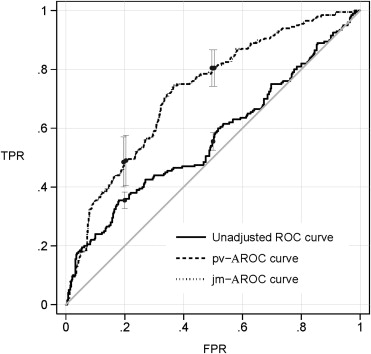
Get Radiology Tree app to read full this article<

Discussion

Get Radiology Tree app to read full this article<

Appendix

Results of additional simulation studies

A.1 Unequal Variance in 50 Cases and 50 Controls

Get Radiology Tree app to read full this article<

Table A.1.1

Average over 1000 Simulated Data Sets of Estimates of Points on the Covariate-Adjusted ROC Curve Calculated with the pv-ROC and jm-ROC Methods Also Shown are the Estimated Covariate-Adjusted AUCs. Data for 50 Cases and 50 Controls were Generated in Each Simulation

μ x μ Y ρ ρ σ0 σ

0 σ1 σ

1 ROC (0.2) ROC (0.5) ROC (0.7) AUC True pv jm True True pv jm True True pv jm True 1 1 0.3 1 1.2 0.464 0.480 0.477 0.730 0.733 0.735 0.853 0.852 0.857 0.681 0.681 0.681 1 1 0.3 1 1.5 0.471 0.485 0.483 0.688 0.692 0.694 0.799 0.802 0.806 0.658 0.658 0.659 1 1 0.3 1 2 0.479 0.488 0.486 0.643 0.648 0.651 0.735 0.738 0.741 0.629 0.629 0.630 1 1 0.5 1 1.2 0.413 0.425 0.423 0.685 0.686 0.688 0.821 0.818 0.822 0.644 0.642 0.643 1 1 0.5 1 1.5 0.430 0.446 0.444 0.650 0.656 0.658 0.769 0.774 0.778 0.626 0.627 0.628 1 1 0.5 1 2 0.447 0.454 0.453 0.614 0.614 0.617 0.709 0.709 0.714 0.602 0.600 0.601 1 1 0.7 1 1.2 0.363 0.380 0.377 0.637 0.643 0.645 0.784 0.785 0.789 0.606 0.606 0.607 1 1 0.7 1 1.5 0.389 0.402 0.402 0.610 0.613 0.618 0.736 0.735 0.743 0.592 0.590 0.594 1 1 0.7 1 2 0.417 0.430 0.433 0.583 0.590 0.595 0.682 0.686 0.693 0.575 0.577 0.582 1 2 0.3 1 1.2 0.783 0.790 0.791 0.931 0.931 0.934 0.973 0.971 0.973 0.873 0.873 0.874 1 2 0.3 1 1.5 0.735 0.742 0.743 0.883 0.882 0.885 0.938 0.938 0.940 0.839 0.838 0.839 1 2 0.3 1 2 0.681 0.695 0.695 0.814 0.818 0.821 0.876 0.879 0.881 0.787 0.792 0.793 1 2 0.5 1 1.2 0.771 0.775 0.776 0.926 0.923 0.926 0.970 0.968 0.970 0.866 0.864 0.866 1 2 0.5 1 1.5 0.724 0.729 0.730 0.876 0.877 0.880 0.934 0.933 0.935 0.832 0.830 0.832 1 2 0.5 1 2 0.672 0.682 0.682 0.807 0.810 0.812 0.870 0.873 0.876 0.781 0.783 0.784 1 2 0.7 1 1.2 0.793 0.796 0.798 0.935 0.934 0.937 0.975 0.973 0.975 0.878 0.878 0.879 1 2 0.7 1 1.5 0.743 0.746 0.748 0.888 0.885 0.887 0.941 0.938 0.941 0.844 0.841 0.842 1 2 0.7 1 2 0.688 0.697 0.696 0.819 0.822 0.824 0.879 0.881 0.884 0.792 0.794 0.795 1.5 1.5 0.3 1 1.2 0.585 0.592 0.594 0.820 0.818 0.820 0.912 0.909 0.914 0.759 0.757 0.758 1.5 1.5 0.3 1 1.5 0.569 0.577 0.578 0.768 0.770 0.773 0.861 0.861 0.863 0.729 0.728 0.729 1.5 1.5 0.3 1 2 0.552 0.563 0.561 0.709 0.715 0.717 0.792 0.795 0.799 0.689 0.691 0.692 1.5 1.5 0.5 1 1.2 0.508 0.528 0.526 0.765 0.768 0.771 0.877 0.876 0.879 0.710 0.711 0.712 1.5 1.5 0.5 1 1.5 0.506 0.519 0.518 0.718 0.718 0.721 0.823 0.822 0.827 0.685 0.684 0.685 1.5 1.5 0.5 1 2 0.505 0.515 0.512 0.667 0.670 0.672 0.757 0.758 0.762 0.651 0.651 0.652 1.5 1.5 0.7 1 1.2 0.430 0.450 0.447 0.700 0.706 0.710 0.832 0.829 0.833 0.657 0.657 0.658 1.5 1.5 0.7 1 1.5 0.444 0.455 0.454 0.663 0.666 0.667 0.779 0.779 0.783 0.637 0.635 0.637 1.5 1.5 0.7 1 2 0.458 0.466 0.465 0.624 0.628 0.629 0.718 0.720 0.724 0.611 0.611 0.612 1.5 2.5 0.3 1 1.2 0.862 0.865 0.868 0.963 0.963 0.965 0.987 0.986 0.987 0.916 0.916 0.917 1.5 2.5 0.3 1 1.5 0.808 0.818 0.820 0.924 0.924 0.927 0.963 0.963 0.965 0.883 0.886 0.887 1.5 2.5 0.3 1 2 0.743 0.749 0.750 0.859 0.861 0.863 0.909 0.910 0.912 0.832 0.831 0.833 1.5 2.5 0.5 1 1.2 0.837 0.840 0.843 0.954 0.954 0.956 0.983 0.983 0.984 0.902 0.902 0.904 1.5 2.5 0.5 1 1.5 0.784 0.791 0.792 0.911 0.910 0.913 0.955 0.954 0.956 0.869 0.868 0.870 1.5 2.5 0.5 1 2 0.722 0.731 0.732 0.844 0.846 0.848 0.898 0.899 0.902 0.817 0.818 0.819 1.5 2.5 0.7 1 1.2 0.839 0.845 0.848 0.955 0.955 0.957 0.983 0.982 0.984 0.903 0.904 0.906 1.5 2.5 0.7 1 1.5 0.786 0.793 0.796 0.912 0.913 0.916 0.956 0.955 0.957 0.870 0.871 0.873 1.5 2.5 0.7 1 2 0.724 0.730 0.731 0.845 0.848 0.849 0.899 0.898 0.901 0.818 0.818 0.819

Table A.1.2

Standard Deviations over 1000 Simulated Data Sets of Estimates of Points on the Covariate-Adjusted ROC Curve and the AUCs Calculated with the pv-ROC and jm-ROC Methods The Relative Efficiency of the New jm method to the Existing pm Method is Quantified by the Ratio of the Variances (var): RE = var(pv)/var(jm). Data for 50 Cases and 50 Controls were Generated in Each Simulation

μ x μ Y ρ ρ σ0 σ

0 σ1 σ

1 ROC (0.2) ROC (0.5) ROC (0.7) AUC pv jm RE pv pv jm RE pv pv jm RE pv 1 1 0.3 1 1.2 0.091 0.092 0.961 0.077 0.077 0.993 0.061 0.060 1.037 0.052 0.052 0.997 1 1 0.3 1 1.5 0.090 0.090 0.993 0.077 0.078 0.970 0.068 0.068 1.018 0.057 0.057 1.011 1 1 0.3 1 2 0.080 0.080 1.007 0.075 0.073 1.050 0.070 0.069 1.047 0.058 0.057 1.046 1 1 0.5 1 1.2 0.094 0.092 1.036 0.087 0.086 1.036 0.070 0.069 1.043 0.057 0.056 1.013 1 1 0.5 1 1.5 0.086 0.087 0.975 0.079 0.079 0.995 0.068 0.068 0.993 0.055 0.055 1.004 1 1 0.5 1 2 0.081 0.081 1.001 0.076 0.075 1.025 0.071 0.071 1.007 0.060 0.058 1.061 1 1 0.7 1 1.2 0.093 0.092 1.028 0.087 0.086 1.022 0.072 0.071 1.025 0.057 0.056 1.035 1 1 0.7 1 1.5 0.087 0.083 1.113 0.083 0.076 1.172 0.074 0.070 1.127 0.060 0.054 1.237 1 1 0.7 1 2 0.080 0.074 1.166 0.078 0.073 1.138 0.076 0.070 1.175 0.060 0.054 1.257 1 2 0.3 1 1.2 0.073 0.074 0.971 0.039 0.039 0.997 0.026 0.026 1.051 0.035 0.035 1.000 1 2 0.3 1 1.5 0.075 0.074 1.031 0.051 0.050 1.006 0.036 0.036 0.993 0.040 0.040 0.996 1 2 0.3 1 2 0.072 0.072 0.991 0.059 0.059 0.995 0.049 0.049 1.022 0.047 0.047 0.998 1 2 0.5 1 1.2 0.074 0.074 1.002 0.044 0.043 1.025 0.028 0.027 1.054 0.036 0.036 0.997 1 2 0.5 1 1.5 0.077 0.078 0.974 0.052 0.052 1.019 0.040 0.039 1.030 0.042 0.042 1.001 1 2 0.5 1 2 0.076 0.076 0.991 0.061 0.060 1.008 0.052 0.050 1.057 0.049 0.049 0.995 1 2 0.7 1 1.2 0.070 0.071 0.982 0.039 0.039 1.016 0.024 0.023 1.102 0.034 0.034 1.000 1 2 0.7 1 1.5 0.077 0.077 0.985 0.052 0.053 0.978 0.038 0.038 1.032 0.042 0.042 1.005 1 2 0.7 1 2 0.074 0.074 0.985 0.058 0.058 1.021 0.049 0.049 1.001 0.046 0.046 1.000 1.5 1.5 0.3 1 1.2 0.093 0.093 0.981 0.066 0.067 0.957 0.048 0.046 1.070 0.047 0.047 1.006 1.5 1.5 0.3 1 1.5 0.085 0.087 0.949 0.067 0.067 0.993 0.054 0.054 0.991 0.050 0.050 0.993 1.5 1.5 0.3 1 2 0.079 0.080 0.963 0.068 0.068 1.013 0.060 0.060 1.004 0.053 0.054 0.993 1.5 1.5 0.5 1 1.2 0.095 0.095 0.991 0.075 0.075 1.008 0.057 0.056 1.022 0.051 0.051 0.998 1.5 1.5 0.5 1 1.5 0.087 0.089 0.942 0.076 0.075 1.015 0.063 0.062 1.016 0.055 0.055 0.992 1.5 1.5 0.5 1 2 0.079 0.079 0.988 0.073 0.073 0.985 0.068 0.068 1.005 0.057 0.057 1.003 1.5 1.5 0.7 1 1.2 0.094 0.095 0.980 0.082 0.081 1.019 0.063 0.064 0.974 0.055 0.055 1.002 1.5 1.5 0.7 1 1.5 0.084 0.085 0.978 0.081 0.081 0.995 0.068 0.068 1.004 0.057 0.056 1.016 1.5 1.5 0.7 1 2 0.078 0.078 1.008 0.074 0.073 1.038 0.069 0.066 1.063 0.057 0.055 1.074 1.5 2.5 0.3 1 1.2 0.061 0.062 0.980 0.028 0.028 1.047 0.017 0.016 1.083 0.028 0.028 1.001 1.5 2.5 0.3 1 1.5 0.065 0.065 1.007 0.042 0.041 1.042 0.030 0.029 1.030 0.034 0.034 1.003 1.5 2.5 0.3 1 2 0.067 0.068 0.974 0.052 0.053 0.976 0.043 0.043 0.999 0.043 0.043 0.989 1.5 2.5 0.5 1 1.2 0.064 0.064 1.002 0.031 0.030 1.055 0.018 0.018 1.036 0.029 0.029 1.011 1.5 2.5 0.5 1 1.5 0.066 0.067 0.967 0.043 0.043 1.034 0.031 0.030 1.045 0.036 0.035 1.014 1.5 2.5 0.5 1 2 0.070 0.071 0.969 0.057 0.056 1.018 0.049 0.048 1.047 0.046 0.046 1.007 1.5 2.5 0.7 1 1.2 0.063 0.062 1.021 0.032 0.032 1.012 0.020 0.019 1.112 0.030 0.030 1.000 1.5 2.5 0.7 1 1.5 0.067 0.069 0.963 0.044 0.043 1.059 0.032 0.030 1.104 0.036 0.036 1.010 1.5 2.5 0.7 1 2 0.070 0.070 0.999 0.053 0.053 1.005 0.045 0.046 0.992 0.043 0.043 0.996

Get Radiology Tree app to read full this article<

A.2 Equal Variance in 20 Cases and 20 Controls

Get Radiology Tree app to read full this article<

Table A.2.1

Average over 1000 Simulated Data Sets of Estimates of Points on the Covariate-Adjusted ROC Curve Calculated with the pv-ROC and jm-ROC Methods Also Shown are the Estimated Covariate-Adjusted AUCs. Data for 20 Cases and 20 Controls were Generated in Each Simulation

_μ__x__μ__Y_ρ ρ ROC (0.2) ROC (0.5) ROC (0.7) AUC True pv jm True pv jm True pv jm True pv jm 1 1 0.3 0.457 0.501 0.500 0.768 0.776 0.786 0.896 0.893 0.902 0.698 0.699 0.702 1 1 0.5 0.396 0.449 0.447 0.718 0.726 0.740 0.865 0.858 0.874 0.658 0.659 0.665 1 1 0.7 0.337 0.394 0.388 0.663 0.676 0.692 0.828 0.825 0.842 0.617 0.619 0.626 1 2 0.3 0.827 0.839 0.847 0.963 0.959 0.963 0.989 0.987 0.990 0.896 0.895 0.899 1 2 0.5 0.813 0.830 0.834 0.958 0.955 0.961 0.988 0.985 0.987 0.890 0.889 0.892 1 2 0.7 0.836 0.850 0.857 0.966 0.963 0.968 0.990 0.988 0.990 0.901 0.903 0.906 1.5 1.5 0.3 0.602 0.638 0.642 0.864 0.859 0.871 0.948 0.942 0.949 0.782 0.783 0.787 1.5 1.5 0.5 0.510 0.548 0.549 0.807 0.805 0.816 0.918 0.909 0.919 0.730 0.728 0.731 1.5 1.5 0.7 0.416 0.463 0.460 0.736 0.744 0.755 0.876 0.875 0.886 0.672 0.673 0.676 1.5 2.5 0.3 0.904 0.908 0.917 0.984 0.981 0.984 0.996 0.994 0.996 0.936 0.936 0.939 1.5 2.5 0.5 0.881 0.888 0.893 0.978 0.976 0.980 0.995 0.993 0.995 0.923 0.923 0.926 1.5 2.5 0.7 0.883 0.887 0.895 0.979 0.977 0.981 0.995 0.994 0.996 0.924 0.925 0.928

Table A.2.2

Standard Deviations over 1000 Simulated Data Sets of Estimates of Points on the Covariate-Adjusted ROC Curve and the AUCs Calculated with the pv-ROC and jm-ROC Methods The Relative Efficiency of the New jm Method to the Existing pm Method is Quantified by the Ratio of the Variances (var): RE = var(pv)/var(jm). Data for 20 Cases and 20 Controls were Generated in Each Simulation

_μ__x__μ__Y_ρ ρ ROC (0.2) ROC (0.5) ROC (0.7) AUC pv jm RE pv jm RE pv jm RE pv jm RE 1 1 0.3 0.162 0.164 0.975 0.123 0.120 1.049 0.084 0.082 1.053 0.084 0.083 1.045 1 1 0.5 0.152 0.153 0.988 0.131 0.122 1.148 0.104 0.094 1.215 0.087 0.081 1.150 1 1 0.7 0.150 0.148 1.024 0.134 0.129 1.080 0.106 0.097 1.192 0.086 0.079 1.204 1 2 0.3 0.109 0.109 0.991 0.050 0.048 1.077 0.026 0.023 1.232 0.049 0.049 1.002 1 2 0.5 0.112 0.112 1.002 0.052 0.051 1.035 0.030 0.027 1.216 0.052 0.052 1.001 1 2 0.7 0.103 0.104 0.981 0.048 0.044 1.177 0.025 0.023 1.219 0.048 0.048 1.009 1.5 1.5 0.3 0.153 0.155 0.967 0.098 0.094 1.081 0.061 0.058 1.101 0.074 0.074 1.003 1.5 1.5 0.5 0.156 0.160 0.959 0.115 0.114 1.019 0.079 0.072 1.211 0.081 0.081 1.013 1.5 1.5 0.7 0.150 0.155 0.936 0.128 0.122 1.096 0.094 0.086 1.178 0.085 0.082 1.057 1.5 2.5 0.3 0.079 0.074 1.129 0.032 0.029 1.186 0.017 0.015 1.271 0.037 0.036 1.026 1.5 2.5 0.5 0.090 0.089 1.037 0.038 0.034 1.205 0.020 0.016 1.448 0.042 0.041 1.024 1.5 2.5 0.7 0.089 0.087 1.049 0.037 0.033 1.232 0.018 0.015 1.444 0.042 0.042 1.003

Get Radiology Tree app to read full this article<

References

1. Gur D., Bandos A.I., Rockette H.E., et. al.: Is an ROC-type response truly always better than a binary response in observer performance studies?. Acad Radiol 2010; vol. 17: pp. 639-645.
2. Samuelson F., Gallas B.D., Myers K.J., et. al.: The importance of ROC data. Acad Radiol 2011; vol. 18: pp. 257-258.
3. Barlow W.E., Chi C., Carney P.A., et. al.: Accuracy of screening mammography interpretation by characteristics of radiologists. J Natl Cancer Inst 2004; vol. 96: pp. 1840-1850.
4. Pepe M., Fan J., Seymour C., et. al.: Biases introduced by choosing controls to match risk factors of cases in biomarker research. Clin Chem 2012; vol. 58: pp. 1242-1251.
5. Janes H., Pepe M.S.: Matching in studies of classification accuracy: implications for analysis, efficiency, and assessment of incremental value. Biometrics 2008; vol. 64: pp. 1-9.
6. Janes H., Pepe M.S.: Adjusting for covariates in studies of diagnostic, screening, or prognostic markers: an old concept in a new setting. Am J Epidemiol 2008; vol. 168: pp. 89-97.
7. Tosteson A.N., Begg C.B.: A general regression methodology for ROC curve estimation. Med Decis Making 1988; vol. 8: pp. 204-215.
8. Faraggi D.: Adjusting receiver operating characteristic curves and related indices for covariates. J R Stat Soc Ser D 2003; vol. 52: pp. 179-192.
9. Zhou X.-H., Obuchowski N.A., McClish D.K.: Regression analysis for independent ROC data.Statistical methods in diagnostic medicine.2011.John Wiley & SonsHoboken, NJ:pp. 261-296.
10. Bossuyt P.M., Reitsma J.B., Bruns D.E., et. al.: Towards complete and accurate reporting of studies of diagnostic accuracy: the STARD initiative. Clin Radiol 2003; vol. 58: pp. 575-580.
11. Pepe M.S., Feng Z., Janes H., et. al.: Pivotal evaluation of the accuracy of a biomarker used for classification or prediction: standards for study design. J Natl Cancer Inst 2008; vol. 100: pp. 1432-1438.
12. Huang Y., Pepe M.: Biomarker evaluation and comparison using the controls as a reference population. Biostatistics 2009; vol. 10: pp. 228.
13. Morris D.E., Pepe M.S., Barlow W.E.: Contrasting two frameworks for ROC analysis of ordinal ratings. Med Decis Making 2010; vol. 30: pp. 484-498.
14. Pepe M.S.: Three approaches to regression analysis of receiver operating characteristic curves for continuous test results. Biometrics 1998; vol. 54: pp. 124-135.
15. Janes H., Longton G., Pepe M.: Accommodating covariates in ROC analysis. Stata J 2009; vol. 9: pp. 17-39.
16. Janes H., Pepe M.S.: Adjusting for covariate effects on classification accuracy using the covariate-adjusted ROC curve. Biometrika 2009; vol. 96: pp. 371-382.
17. Kerr K.F., Pepe M.S.: Joint modeling, covariate adjustment, and interaction: contrasting notions in risk prediction models and risk prediction performance. Epidemiology 2011; vol. 22: pp. 805-812.
18. Pepe M.S.: The statistical evaluation of medical tests for classification and prediction.2003.Oxford University PressOxford, UK
19. Seymour C.W., Kahn J.M., Cooke C.R., et. al.: Prediction of critical illness during out-of-hospital emergency care. JAMA 2010; vol. 304: pp. 747-754.
20. Parikh C.R., Devarajan P., Zappitelli M., et. al.: Postoperative biomarkers predict acute kidney injury and poor outcomes after pediatric cardiac surgery. J Am Soc Nephrol 2011; vol. 22: pp. 1737-1747.

Estimating the Receiver Operating Characteristic Curve in Studies That Match Controls to Cases on Covariates

Rationale and Objectives

Materials and Methods

Results

Conclusions

Materials and methods

The Covariate-Adjusted ROC Curve

Existing Estimator of the AROC: The pv -AROC Estimator

A New Method for Matched Data: The jm -AROC Estimator

Rationale for the jm -AROC Estimator

Result

Data and Estimation Details for Simulation Studies

Data on a Diagnostic Test for Critical Illness

Results

Results from Illustrative Data Sets

Bias and Efficiency of Estimators in Simulated Data

Application to Diagnostic Tests for Critical Illness

Discussion

Appendix

Results of additional simulation studies

A.1 Unequal Variance in 50 Cases and 50 Controls

A.2 Equal Variance in 20 Cases and 20 Controls

References

Further Reading

A Brief History of Free-Response Receiver Operating Characteristic Paradigm Data Analysis

An Additive Selection of Markers to Improve Diagnostic Accuracy Based on a Discriminatory Measure

An Examination of Data Confidentiality and Disclosure Issues Related to Publication of Empirical ROC Curves