
Rationale and Objectives
Accurate classification is critical in mammography computer-aided diagnosis using content-based image retrieval approaches (CBIR CAD). The objectives of this study were to: 1) develop an accurate ensemble classifier based on domain knowledge and a robust feature selection method for CBIR CAD; 2) propose three new features; and 3) assess the performance of the proposed method and new features by using a relatively large imaging data set.
Materials and Methods
The data set used in this study consisted of 2114 regions of interest (ROI) extracted from a publicly available image database. The proposed ensemble classifier method we called E-DGA-KNN included four steps. In the first step, 804 ROIs depict masses were divided into five classes according to their boundary types. Then, each class of ROI with an equal number of negative ROIs were put together to create a sub-database. Second, a dual-stage genetic algorithm, which was called DGA, was applied on those five sub-databases for feature selection and weights determination respectively. In the third step, five base K-nearest neighbor (KNN) classifiers were created by using the results of the second step on 2114 ROIs, and five detection scores for a given queried ROI were obtained. Finally, these classifiers are combined to yield a final classification. The performances of the proposed methods were evaluated by using receiver operating characteristic (ROC) analysis. A comparison with eight different methods on the data set was provided which include the stepwise linear discriminative analysis algorithm (SLDA) and particle swarm optimization (PSO) algorithm with KNN classifier.
Results
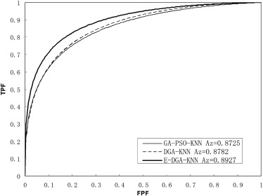
When four hybrid feature selection methods were applied with single KNN classifier (ie, DGA-KNN, SLDA-WGA-KNN, SLDA-PSO-KNN, GA-PSO-KNN) and the proposed E-DGA-KNN method to the data set, the computed areas under the ROC curve (Az) were 0.8782 ± 0.0080, 0.8675 ± 0.0081, 0.8623 ± 0.0083, 0.8725 ± 0.0079, and 0.8927 ± 0.0073, respectively. If all features and single KNN classifier were used, the Az value was 0.8478 ± 0.0088. Az values were 0.8592 ± 0.0083 and 0.8632 ± 0.0081 when SLDA or GA algorithm used alone.
Conclusions
In this study, an ensemble classifier based on domain knowledge and a dual-stage feature selection method was proposed. Evaluation results indicated that the proposed method achieved largest value of ROC compared to other algorithms. The proposed method shows better performance and has the potential to improve the performance of CBIR CAD in interpreting and analyzing mammograms.
Breast cancer is still one of the most common classes of cancer among women all over the world . Early detection of breast cancer plays a major role in reducing mortality. Mammography is widely regarded as the most effective tool for breast cancer early detection and diagnosis available today . However, mammogram interpretation is a difficult and error-prone task. To aid radiologists in reading mammograms, many researchers have developed computer-aided diagnosis (CAD) systems . At present, researches are focusing on developing mammography CAD scheme using content-based image retrieval approaches (CBIR CAD) .
The goal of CBIR CAD scheme is to detect whether and what degree the queried region of interest (ROI) similar to breast masses. In other words, the CBIR CAD scheme will retrieve K reference ROIs most similar to the queried ROI. It gives visual aids and a number of relative information to radiologists. For the time being, there are two typical types of CBIR CAD that have been developed in mammography: multifeature-based K-nearest neighbor (KNN) methods and template matching–based methods . In this study, we focus on the former, which yields significantly higher performance than the latter that was demonstrated by Wang et al .
Get Radiology Tree app to read full this article<
Get Radiology Tree app to read full this article<
Get Radiology Tree app to read full this article<
Materials and methods
Overview
Get Radiology Tree app to read full this article<
Get Radiology Tree app to read full this article<
Reference-image Database
Get Radiology Tree app to read full this article<
Table 1
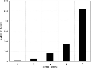
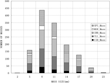
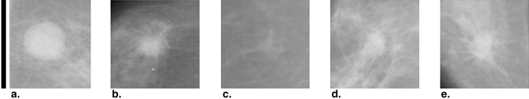
Detailed Distribution of ROIs Depict Mass
Digitizer CIR MIR ILL IRR SPI Howtek 32 6 193 202 114 Lumisys 76 72 181 228 206 Total 108 78 374 430 320
CIR, circumscribed; ILL, ill-defined; IRR, irregular; MIR, microlobulated; ROIs, regions of interest; SPI, spiculated.
Get Radiology Tree app to read full this article<
Get Radiology Tree app to read full this article<
Get Radiology Tree app to read full this article<
Get Radiology Tree app to read full this article<
Get Radiology Tree app to read full this article<
Get Radiology Tree app to read full this article<
Get Radiology Tree app to read full this article<
Masses Segmentation
Get Radiology Tree app to read full this article<
Feature Extraction and Computation
Get Radiology Tree app to read full this article<
Feature 1: Correlation coefficient between Gauss template and the central region of ROI
Get Radiology Tree app to read full this article<
Z(x,y)=12πσ2exp(−x2+y22σ2) Z
(
x
,
y
)
=
1
2
π
σ
2
exp
(
−
x
2
+
y
2
2
σ
2
)
Get Radiology Tree app to read full this article<
Get Radiology Tree app to read full this article<
Coeff=∑−R2≤x,y≤R2(G(x,y)−G¯¯¯)(Z(x,y)−Z¯¯¯)∑−R2≤x,y≤R2(G(x,y)−G¯¯¯)2√∑−R2≤x,y≤R2(Z(x,y)−Z¯¯¯)2√ C
o
e
f
f
=
∑
−
R
2
≤
x
,
y
≤
R
2
(
G
(
x
,
y
)
−
G
¯
)
(
Z
(
x
,
y
)
−
Z
¯
)
∑
−
R
2
≤
x
,
y
≤
R
2
(
G
(
x
,
y
)
−
G
¯
)
2
∑
−
R
2
≤
x
,
y
≤
R
2
(
Z
(
x
,
y
)
−
Z
¯
)
2
where G(x,y) G
(
x
,
y
) is a sub-image of ROI whose height and weight are equal to the Gauss template.
Get Radiology Tree app to read full this article<
Feature 2: Gauss template relative coefficient of gravity center of mass
Get Radiology Tree app to read full this article<
Feature 3: Euclidean distance between ROI center and gravity center of segmented region
Get Radiology Tree app to read full this article<
The Proposed Ensemble Classifier Based on Domain Knowledge and a Dual-stage Feature Selection Method
Get Radiology Tree app to read full this article<
Get Radiology Tree app to read full this article<
Get Radiology Tree app to read full this article<

Get Radiology Tree app to read full this article<
Step 1: Create five sub-databases with feature description
Get Radiology Tree app to read full this article<
Step 2: Using the proposed dual-stage method to search for corresponding feature subsets and weights on each sub-database
Get Radiology Tree app to read full this article<
Stage 1: Acquire a candidate feature subset using conventional GA
Get Radiology Tree app to read full this article<
The Way of Individual Coding
Get Radiology Tree app to read full this article<
Table 2
Individual Coding in Genetic Algorithms
Features Part Neighbors Number Part g 1 g 2 … g v g v+1 g v+2 … g v+u f 1 f 2 … f v u bits for K in KNN
Get Radiology Tree app to read full this article<
The Design of Fitness Function
Get Radiology Tree app to read full this article<
The Design of the Generic Operators
Get Radiology Tree app to read full this article<
Stage 2: Acquire the weights of features using weighted WGA on basis of stage 1
Get Radiology Tree app to read full this article<
Table 3
Individual Coding in Weighted Genetic Algorithms
Features Part Neighbors Number Part g 11 g 12 … g 1t … g n1 g n2 … g nt g nt +1 … g nt +u’ Weight of f 1 … Weight of f n u’ bits for K in KNN
Get Radiology Tree app to read full this article<
Get Radiology Tree app to read full this article<
Step 3: Create base classifiers
Get Radiology Tree app to read full this article<
Get Radiology Tree app to read full this article<
Sim(X,Y)=1d(X,Y)=1∑Fr=1wr(fr(X)−fr(Y))2√ S
i
m
(
X
,
Y
)
=
1
d
(
X
,
Y
)
=
1
∑
r
=
1
F
w
r
(
f
r
(
X
)
−
f
r
(
Y
)
)
2
where F is a multidimensional feature space and fr f
r is the r- th selected feature.
Get Radiology Tree app to read full this article<
Get Radiology Tree app to read full this article<
DI(X)=∑Ki=1,Yi∈Mass(Sim(X,Yi)×(k+1−R(Yi)))∑Ki=1(Sim(X,Yi)×(k+1−R(Yi))) D
I
(
X
)
=
∑
i
=
1
,
Y
i
∈
M
a
s
s
K
(
S
i
m
(
X
,
Y
i
)
×
(
k
+
1
−
R
(
Y
i
)
)
)
∑
i
=
1
K
(
S
i
m
(
X
,
Y
i
)
×
(
k
+
1
−
R
(
Y
i
)
)
)
Where, R (Y i ) is the descending sort order of the i- th ROI according to the similarity. It is obvious that a larger DI indicates that a larger probability of the queried ROI being a true-positive mass.
Get Radiology Tree app to read full this article<
Step 4: Create ensemble classifier
Get Radiology Tree app to read full this article<
PTP(ROIj)=∑5i=1qiDIi(ROIj),i∈(1,2⋯5),j∈(1,2⋯2114) P
T
P
(
R
O
I
j
)
=
∑
i
=
1
5
q
i
D
I
i
(
R
O
I
j
)
,
i
∈
(
1
,
2
⋯
5
)
,
j
∈
(
1
,
2
⋯
2114
)
where qi=Number(MassTypei)Number(MassTotal) q
i
=
N
u
m
b
e
r
(
M
a
s
s
T
y
p
e
i
)
N
u
m
b
e
r
(
M
a
s
s
T
o
t
a
l
) , and DIi(ROIj) D
I
i
(
R
O
I
j
) represented the decision scores of j- th ROI by the i- th base classifier.
Get Radiology Tree app to read full this article<
Results
Get Radiology Tree app to read full this article<
Table 4
Experimental Results
Methods Number of Selected Features K Az SE 95% Confidence Intervals AF-KNN 63 58 0.8478 0.0088 0.8298–0.8644 GA-KNN 34 58 0.8632 0.0081 0.8463–0.8788 SLDA-KNN 26 58 0.8592 0.0083 0.8422–0.8749 GA-PSO-KNN 22 58 0.8725 0.0079 0.8562–0.8874 SLDA-PSO-KNN 14 58 0.8623 0.0083 0.8454–0.8779 SLDA-WGA-KNN 21 58 0.8675 0.0081 0.8510–0.8827 DGA-KNN 24 59 0.8782 0.0078 0.8612–0.8942 E-DGA-KNN ∗ 14/9/15/7/13 31/30/49/36/61 0.8927 0.0073 0.8794–0.9073
Get Radiology Tree app to read full this article<
Get Radiology Tree app to read full this article<
Get Radiology Tree app to read full this article<
Get Radiology Tree app to read full this article<
Get Radiology Tree app to read full this article<
Table 5
Statistical Analysis Results
Analysis Method E-DGA-KNN and DGA-KNN E-DGA-KNN and GA-KNN DGA-KNN and GA-KNN Correlation 0.9200 0.8959 0.9517 Bivariate V 19.1883 39.1408 16.6943P .0001 <.0001 .0002 Area V 4.2585 6.1566 3.5437 1- P <.0001 <.0001 .0002 2- P <.0001 <.0001 .0004 CI 0.0072–0.0196 0.0158–0.0306 0.0041–0.0141 True-positive fraction V −4.3668 −3.8590 −3.5332 1- P <.0001 .0001 .0002 2- P <.0001 .0001 .0004 CI −0.0396 to −0.0088 −0.0515 to 0.0408 −0.0365 to 0.0299
See Table 6 for definitions.
Table 6
Definitions of Values
Symbol Meaning Bivariate (V) Value of computed correlated bivariate chi-square test statistic Bivariate ( P ) Corresponding P value Area (V) Value of computed correlated area test statistic Area (1-P) Corresponding one-tailed P value Area (2- P ) Corresponding two-tailed P value Area (CI) Approximate 95% Confidence Interval for the difference TPF (V) Value of computed correlated true-positive fraction test statistic TPF (1- P ) Corresponding one-tailed P value TPF (2- P ) Corresponding two-tailed P value TPF (CI) Approximate 95% confidence interval for the difference
Get Radiology Tree app to read full this article<
Get Radiology Tree app to read full this article<
Table 7
Results of Each Experiment after Two Stages on Each Sub-database
Sub-database First Stage (GA) Second Stage (DGA) Az K Az K CIR 0.9136 ± 0.0081 32 0.9609 ± 0.0080 31 ILL 0.8407 ± 0.0079 38 0.8596 ± 0.0082 30 IRR 0.8421 ± 0.0080 35 0.8685 ± 0.0077 49 MIR 0.9460 ± 0.0082 44 0.9493 ± 0.0083 36 SPI 0.8657 ± 0.0081 58 0.8981 ± 0.0082 61
CIR, circumscribed; ILL, ill-defined; IRR, irregular; MIR, microlobulated; ROIs, regions of interest; SPI, spiculated.
Get Radiology Tree app to read full this article<
Get Radiology Tree app to read full this article<
N(X)=argimax(DIi(X)),1≤i≤5 N
(
X
)
=
arg
i
max
(
D
I
i
(
X
)
)
,
1
≤
i
≤
5
Table 8
The Maximum Decision Score Distribution for Each Class of Masses
ROIs CIR ILL IRR MIR SPI Total CIR ROIs 56 26 8 15 3 108 ILL ROIs 6 171 143 30 24 374 IRR ROIs 10 150 187 11 72 430 MIR ROIs 2 15 12 41 8 78 SPI ROIs 10 98 77 6 129 320
CIR, circumscribed; ILL, ill-defined; IRR, irregular; MIR, microlobulated; ROIs, regions of interest; SPI, speculated.
Get Radiology Tree app to read full this article<
Get Radiology Tree app to read full this article<
F(m,i)=∑X∈m−thclassofROIsδ(N(X)−i),1≤i≤5,1≤m≤5 F
(
m
,
i
)
=
∑
X
∈
m
−
t
h
class
of
R
O
I
s
δ
(
N
(
X
)
−
i
)
,
1
≤
i
≤
5
,
1
≤
m
≤
5
where δ(n)={10ifn=0else δ
(
n
)
=
{
1
i
f
n
=
0
0
e
l
s
e .
Get Radiology Tree app to read full this article<
Get Radiology Tree app to read full this article<
Get Radiology Tree app to read full this article<
Table 9
Weights of Proposed Features in Feature Selection Methods
Selection Methods Weights of the Proposed Features Feature 1 Feature 2 Feature 3 GA 1 1 1 SLDA 1 1 0 DGA 0.0282 0.0563 0.0282 SLDA-WGA 0.0694 0.0107 0 GA-PSO 0.0069 0.0019 0.0143 SLDA-PSO 0.077 0 0
Table 10
Weights of Proposed Features in Each Sub-database in E-DGA-KNN
Sub-database Weights of Proposed Features Feature 1 Feature 2 Feature 3 CIR 0 0 0 ILL 0.1296 0.1806 0 IRR 0.0131 0.0521 0 MIR 0.1434 0 0 SPI 0.0663 0 0.0549
CIR, circumscribed; ILL, ill-defined; IRR, irregular; MIR, microlobulated; ROIs, regions of interest; SPI, speculated.
Get Radiology Tree app to read full this article<
Discussion
Get Radiology Tree app to read full this article<
Get Radiology Tree app to read full this article<
Get Radiology Tree app to read full this article<
Get Radiology Tree app to read full this article<
Get Radiology Tree app to read full this article<
Conclusions
Get Radiology Tree app to read full this article<
Get Radiology Tree app to read full this article<
References
1. Shi J., Sahiner B., Chan H.P., et. al.: Characterization of mammographic masses based on level set segmentation with new image features and patient information. Med Phys 2008; 35: pp. 280-290.
2. Kinnard L., Lo S.C.B., Makariou E., et. al.: Steepest changes of a probability-based cost function for delineation of mammographic masses: a validation study. Med Phys 2004; 31: pp. 2796-2810.
3. Suliga M., Deklerck R., Nyssen E.: Markov random field-based clustering applied to the segmentation of masses in digital mammograms. Comp Med Imaging Graphics 2008; 32: pp. 502-512.
4. Ko J.M., Nicholas M.J., Mendel J.B., et. al.: Prospective assessment of computer-aided detection in interpretation of screening mammography. AJR Am J Roentgenol 2006; 187: pp. 1483-1491.
5. Menotti M., Lanconelli N., Campanini R.: Computer-aided mass detection in mammography: false positive reduction via gray-scale invariant ranklet texture features. Med Phys 2009; 36: pp. 311-316.
6. Zheng B, Abrams G, Britton CA, et al. Evaluation of an interactive computer-aided diagnosis (ICAD) system for mammography: a pilot study. Presented at Proc. SPIE 6515, 65151M; 2007.
7. Yimo T. A preliminary study of content-based mammographic masses retrieval. Presented at Proc. SPIE 6514, 65141Z; 2007.
8. Zheng B., Mello-Thoms C., Wang X.H., et. al.: Interactive Computer-aided diagnosis of breast masses: computerized selection of visually similar image sets from a reference library. Acad Radiol 2007; 14: pp. 917-927.
9. Tourassi G.D., Vargas-Voracek R., Catarious D.M., et. al.: Computer-assisted detection of mammographic masses: a template matching scheme based on mutual information. Med Phys 2003; 30: pp. 2123-2130.
10. Filev P., Hadjiiski L., Sahiner B., et. al.: Comparison of similarity measures for the task of template matching of masses on serial mammograms. Med Phys 2005; 32: pp. 515-529.
11. Wang X.H., Park S.C., Zheng B.: Improving performance of content-based image retrieval schemes in searching for similar breast mass regions: an assessment. Phys Med Biol 2009; 54: pp. 949-961.
12. Kupinski M.A., Giger M.L.: Feature selection with limited datasets. Med Phys 1999; 26: pp. 2176-2182.
13. Soltanian-Zadeh H., Rafiee-Rad F., Pourabdollah-Nejad D.: Comparison of multiwavelet, wavelet, Haralick, and shape features for microcalcification classification in mammograms. Pattern Recognition 2004; 37: pp. 1973-1986.
14. Chan H.P., Sahiner B., Lam K.L., et. al.: Computerized analysis of mammographic microcalcifications in morphological and texture feature spaces. Med Phys 1998; 25: pp. 2007-2019.
15. Zheng B., Lu A., Hardesty L.A., et. al.: A method to improve visual similarity of breast masses for an interactive computer-aided diagnosis environment. Med Phys 2006; 33: pp. 111-117.
16. Catarious D.M., Baydush A.H., Floyd C.E.: Incorporation of an iterative, linear segmentation routine into a mammographic mass CAD system. Med Phys 2004; 31: pp. 1512-1520.
17. Pranckeviciene E., Baumgartner R., Somorjai R.: Using domain knowledge for in the random subspace method: application: application to the classification of biomedical spectra. Multiple Classifier Sys 2005; 3541: pp. 336-345.
18. Lee M.C., Boroczky L., Sungur-Stasik K., et. al.: Computer-aided diagnosis of pulmonary nodules using a two-step approach for feature selection and classifier ensemble construction. Artific Intell Med 2010; 50: pp. 43-53.
19. Yu E., Cho S.: Ensemble based on GA wrapper feature selection. Comp Industrial Eng 2006; 51: pp. 111-116.
20. Renchao J, Bo M, Enmin S, et al. Computer-aided detection of mammographic masses based on content-based image retrieval. Presented at: Medical Imaging: Computer-Aided Diagnosis. Bellingham, WA; 2007.
21. Efron B., Tibshirani R.J.: An introduction to the bootstrap: monographs on statistics and applied probability1998.Chapman and HallNew York
22. Park S.C., Wang X.H., Zheng B.: Assessment of performance improvement in content-based medical image retrieval schemes using fractal dimension. Acad Radiol 2009; 16: pp. 1171-1178.
23. Heath M., Bowyer K., Kopans D., et. al.: Current status of the digital database for screening mammography. Comput Imaging Vision 1998; 13: pp. 457-460.
24. Heath M, Bowyer K, Kopans D, et al. The digital database for screening mammography. Presented at: 5th International Workshop on Digital Mammography; June 2000; Toronto, Canada.
25. Rojas Domínguez A., Nandi A.K.: Improved dynamic-programming-based algorithms for segmentation of masses in mammograms. Med Phys 2007; 34: pp. 4256-4269.
26. Enmin X., Shengzhou X., Xiangyang X., et. al.: Hybrid segmentation of mass in mammograms using template matching and dynamic programming. Acad Radiol 2010; 17: pp. 1414-1424.
27. Zheng B., Sumkin J.H., Good W.F., et. al.: Applying computer-assisted detection schemes to digitized mammograms after JPEG data compression: an assessment. Acad Radiol 2000; 7: pp. 595-602.
28. Zheng B., Lu A., Hardesty L.A., et. al.: A method to improve visual similarity of breast masses for an interactive computer-aided diagnosis environment. Med Phys 2006; 33: pp. 111-117.
29. Petrick N., Chan H.-P., Wei D., et. al.: Automated detection of breast masses on mammograms using adaptive contrast enhancement and texture classification. Med Phys 1996; 23: pp. 1685-1695.
30. Jiang L., Song E., Xu X., et. al.: Automated detection of breast mass spiculation levels and evaluation of scheme performance. Acad Radiol 2008; 15: pp. 1534-1544.
31. Catarious D.M., Baydush A.H., Floyd C.E.: Characterization of difference of Gaussian filters in the detection of mammographic regions. Med Phys 2006; 33: pp. 4104-4114.
32. Yang J., Honavar V.: Feature subset selection using a genetic algorithm. Intelligent Systems and Their Applications. IEEE 1998; 13: pp. 44-49.