
Rationale and Objectives
Thinned perforator flaps have been widely used in plastic surgery for greater survivability and decreased morbidity. However, quantitative analysis of three-dimensional (3D) blood flow direction and location has not been examined yet. Such information will benefit and guide the surgical thinning and dissection process. Toward this goal, this study was performed for 3D vascular tree reconstruction with the incorporation of temporal contrast-agent propagation information (three spatial dimensions plus one temporal dimension; ie, 4D).
Materials and Methods
A novel computational framework by adopting a moving grid deformation method is presented. To take advantage of temporal information of the bolus propagating, a sequential segmentation procedure is proposed. Moreover, the temporal evolution of the vascular tree (4D vascular tree) is reconstructed during the procedure.
Results
Eight anterolateral thigh perforator flaps from eight cadavers were used for this study. The age range is 60–80 years old and the gender includes four males and four females. The 3D nature of the vascular structure and 4D vascular tree evolving process are showed in comparison with maximum intensity projection images.
Conclusion
The proposed computational framework demonstrates effectiveness in the modeling of 4D vascular tree. Furthermore, it reveals the ability to detect small vessel tree structures that are beyond the limit of image resolution.
Perforator flaps have been increasingly used over the past decade in plastic surgery for greater survivability and decreased morbidity ( ). The majority of anatomic vascular studies on perforator flaps have used lead oxide injections on cadaver flaps followed by two-dimensional (2D) projection radiography to determine vascular territories. Although lead oxide treated specimens provide excellent images, the three-dimensional (3D) nature of the vascular structure is not revealed. To overcome this deficit, static computed tomography (CT) scanning can be used to provide 3D mappings of contrast enhanced vascular anatomy in the sagittal, coronal, and transverse views. However, none of these methods can provide insight information on the direction and location of blood flow within each layer of a perforator flap. In this study, we present a four-dimensional (4D) (ie, three spatial dimensions plus one temporal dimension) time sequence of perforator flaps showing the process of contrast agent propagation. To our best knowledge, no study has been carried out reporting the examination of 4D anatomy of perforator flaps.
The computational techniques used in traditional 3D vasculature tree reconstruction ( ) can be roughly grouped into six categories ( ): 1) pattern recognition techniques; 2) model-based approaches; 3) tracking-based approaches; 4) artificial intelligence–based approaches; 5) neural network–based approaches; and 6) miscellaneous tubelike object detection approaches. Unfortunately, no single method works for any applications. The most widely used model-based methods in vessel reconstruction are the geometric deformable models. One problem with geometric deformable models is the high computational cost. To improve the efficiency and accuracy, adaptive grid techniques have been adopted ( ) to help solve the partial differential equations involved in geometric deformable models.
Get Radiology Tree app to read full this article<
Get Radiology Tree app to read full this article<
Materials and methods
Get Radiology Tree app to read full this article<
CT Radiography
Get Radiology Tree app to read full this article<
Get Radiology Tree app to read full this article<
Get Radiology Tree app to read full this article<
Moving Grid Generation by Deformation Method
Get Radiology Tree app to read full this article<
Get Radiology Tree app to read full this article<
Get Radiology Tree app to read full this article<
Get Radiology Tree app to read full this article<
Step 1
Get Radiology Tree app to read full this article<
Get Radiology Tree app to read full this article<
divv→(xt,yt,t)=−∂∂t(1m(,t)), d
i
v
v
→
(
x
t
,
y
t
,
t
)
=
−
∂
∂
t
(
1
m
(
,
t
)
)
,
Get Radiology Tree app to read full this article<
Get Radiology Tree app to read full this article<
curlv→(xt,yt,t)=0, c
u
r
l
v
→
(
x
t
,
y
t
,
t
)
=
0
,
Get Radiology Tree app to read full this article<
Get Radiology Tree app to read full this article<
v→(xt,yt,t)⋅n→=0,for(xt,yt)∈∂Ω(t), v
→
(
x
t
,
y
t
,
t
)
⋅
n
→
=
0
,
f
o
r
(
x
t
,
y
t
)
∈
∂
Ω
(
t
)
,
where ∂Ω(t) ∂
Ω
(
t
) denotes the boundary of domain Ω(t) Ω
(
t
) . The Neumann boundary condition specifies the values the derivatives of a solution is to take on the boundary of the domain. In an image domain, the boundary constraint is zero which means the boundary points cannot move out or move inside to the image domain, but only move along the boundary. This is reflected as the zero vector field in the normal direction as shown in Eq 3 .
Get Radiology Tree app to read full this article<
Get Radiology Tree app to read full this article<
Get Radiology Tree app to read full this article<
divv→(x,y,t)=∇⋅v→(x,y,t), d
i
v
v
→
(
x
,
y
,
t
)
=
∇
⋅
v
→
(
x
,
y
,
t
)
,
Get Radiology Tree app to read full this article<
Get Radiology Tree app to read full this article<
curlv→(x,y,t)=∇×v→(x,y,t). c
u
r
l
v
→
(
x
,
y
,
t
)
=
∇
×
v
→
(
x
,
y
,
t
)
.
Get Radiology Tree app to read full this article<
Get Radiology Tree app to read full this article<
Step 2
Get Radiology Tree app to read full this article<
Get Radiology Tree app to read full this article<
∂∂t(x,y,t)=m((x,y,t),t)v→((x,y,t),t), ∂
∂
t
(
x
,
y
,
t
)
=
m
(
(
x
,
y
,
t
)
,
t
)
v
→
(
(
x
,
y
,
t
)
,
t
)
,
where t∈[0,T] t
∈
[
0
,
T
] .
Get Radiology Tree app to read full this article<
Get Radiology Tree app to read full this article<
∫Ω(t)(−∂∂t(1m(,t)))dxdy=0 ∫
Ω
(
t
)
(
−
∂
∂
t
(
1
m
(
,
t
)
)
)
d
x
d
y
=
0
for all t . Furthermore, the monitor function m(,t) m
(
,
t
) should be normalized under the following condition,
Get Radiology Tree app to read full this article<
Get Radiology Tree app to read full this article<
∫Ω(t)1m(,t)dxdy=|Ω(0)|,forallt, ∫
Ω
(
t
)
1
m
(
,
t
)
d
x
d
y
=
|
Ω
(
0
)
|
,
for
all
t
,
where | Ω(0) | means the area over the domain Ω at time t = 0. The mathematical proof of the deformation method can be found elsewhere ( ).
Get Radiology Tree app to read full this article<
Vascular Tree Reconstruction using Moving Grid with Deformation
Get Radiology Tree app to read full this article<
Initial segmentation
Get Radiology Tree app to read full this article<
Vascular grid plot generation
Get Radiology Tree app to read full this article<
m0()={0.3,whenpoint(x,y)belongstoinitialsegmentedvesselregion;1.0,else m
0
(
)
=
{
0.3
,
when
point
(
x
,
y
)
belongs
to
initial
segmented
vessel
region
;
1.0
,
else
Get Radiology Tree app to read full this article<
Get Radiology Tree app to read full this article<
Get Radiology Tree app to read full this article<
m(,t)=1−tT+tT⋅m0(), m
(
,
t
)
=
1
−
t
T
+
t
T
⋅
m
0
(
)
,
where t∈[0,T] t
∈
[
0
,
T
] is the dummy time variable used in the grid deformation process same as the one occurred in Eq 1–7 . By this definition, we have m(,0)=1 m
(
,
0
)
=
1 and m(,T)=m0() m
(
,
T
)
=
m
0
(
) . This implies the grid is deformed from uniform to the desired one in which the size of a grid cell is governed by the objective monitor function m0() m
0
(
) . The normalization of m(,t) m
(
,
t
) is carried out using Eq 7 for all t∈[0,T] t
∈
[
0
,
T
] .
Get Radiology Tree app to read full this article<
Get Radiology Tree app to read full this article<
Vascular vessel extraction
Get Radiology Tree app to read full this article<
Get Radiology Tree app to read full this article<
Get Radiology Tree app to read full this article<
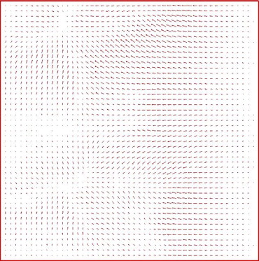
v→T=<xT−x0,yT−y0>T, v
→
T
=
<
x
T
−
x
0
,
y
T
−
y
0
T
,
where (x0,y0) (
x
0
,
y
0
) is the initial uniform grid, and (xT,yT) (
x
T
,
y
T
) is the grid plot using the deformation method.
Get Radiology Tree app to read full this article<
Get Radiology Tree app to read full this article<
Get Radiology Tree app to read full this article<
F(xT,yT)=∇⋅v→T. F
(
x
T
,
y
T
)
=
∇
⋅
v
→
T
.
Get Radiology Tree app to read full this article<
Get Radiology Tree app to read full this article<
Results
Get Radiology Tree app to read full this article<
Demonstration of the Proposed Method
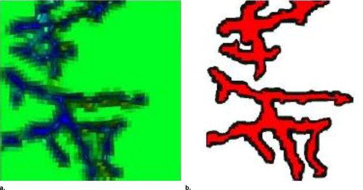
Initial vascular tree segmentation
Get Radiology Tree app to read full this article<
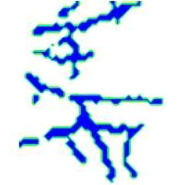
Get Radiology Tree app to read full this article<
Get Radiology Tree app to read full this article<
Get Radiology Tree app to read full this article<
Grid plot generation
Get Radiology Tree app to read full this article<
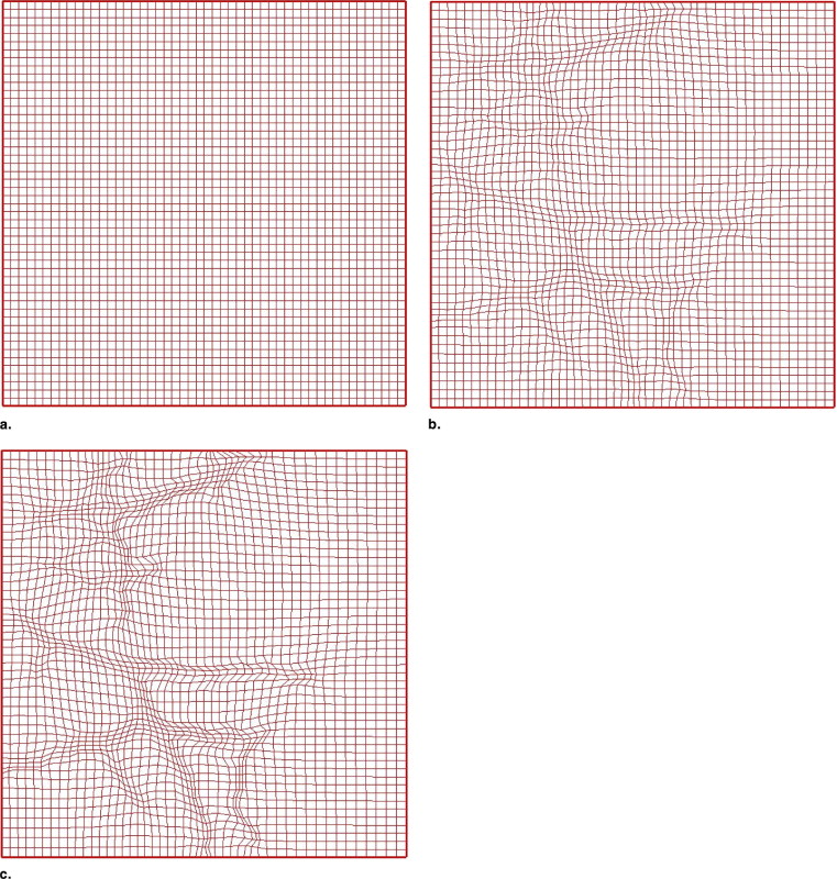
Get Radiology Tree app to read full this article<
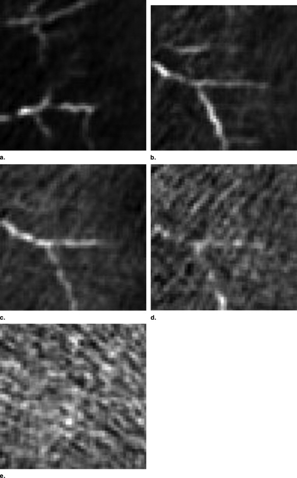
Vascular vessel extraction
Get Radiology Tree app to read full this article<
Get Radiology Tree app to read full this article<
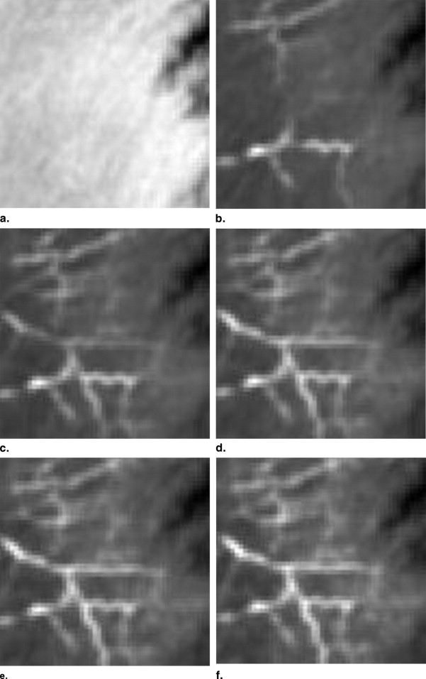
4D vascular tree evolution
Get Radiology Tree app to read full this article<
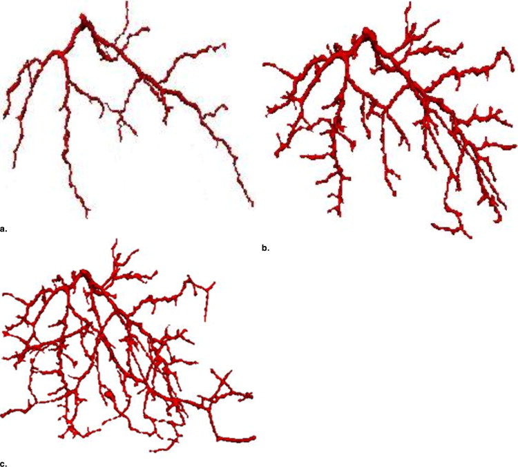
Get Radiology Tree app to read full this article<
Results for Datasets ALT2-ALT8
Get Radiology Tree app to read full this article<
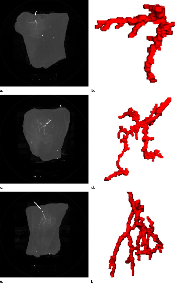
Get Radiology Tree app to read full this article<
Discussion
Get Radiology Tree app to read full this article<
Get Radiology Tree app to read full this article<
Get Radiology Tree app to read full this article<
Get Radiology Tree app to read full this article<
Get Radiology Tree app to read full this article<
Get Radiology Tree app to read full this article<
Get Radiology Tree app to read full this article<
References
1. Allen R.J., Treece P.: Deep inferior epigastric perforator flap for breast reconstruction. Ann Plastic Surg 1994; 32: pp. 32-38.
2. Wei C., Jain V., Suominen S., Chen H.: Confusion among perforator flap: what is a true perforator flap?. Plastic Reconstr Surg 2001; 107: pp. 874-876.
3. Abdul-Karim M.A., Roysam B., Dowell-Mesfin N.M., et. al.: Automatic selection of parameters for vessel/neurite segmentation algorithms. IEEE Trans Image Proc 2005; 14: pp. 1338-1350.
4. Condurache A.P., Aach T., Grzybowski S., et. al.: Imaging and analysis of angiogennesis for skin transplantation by microangiography. Proc IEEE Conf Image Proc 2005; 2: pp. 1250-1253.
5. Passat N., Ronse C., Baruthio J., et. al.: Cerebral vascular atlas generation for anatomical knowledge modeling and segmentation purpose. Proc Computer Vision Patteren Recognit 2005; 2: pp. 331-337.
6. Sebbe R., Gosselin B., Coche E., et. al.: Model-guided segmentation of opacified thorax vessels. Proc IEEE Conf Image Proc 2005; 1: pp. 25-28.
7. Sekiguchi H., Sugimoto N., Eiho S., et. al.: Blood vessel segmentation for head MRA using branch-based region growing. Syst Computers Jap 2005; 36: pp. 5.
8. Kirbas C., Quek F.K.H.: Vessel extraction techniques and algorithms: a survey. Proc IEEE Symp BioInfor BioEng 2003; 4: pp. 238-245.
9. Droske M., Meyer B., Schaller C., et. al.: An adaptive level set method for medical image segmentation. Proceedings of the International Conference on Information Processing in Medical Image 2001; 2080: pp. 416-422.
10. Han X., Xu X., Prince J.P.: A 2D moving grid geometric deformable model. Proc Computer Vision Patteren Recognit 2003; 1: pp. 153.
11. Xue J., Liao G.: Least-squares finite element method on adaptive grid for PDEs with shocks. Numer Meth Part Diff Eq 2006; 22: pp. 114-127.
12. Zegeling P.A.: Moving grid techniques.Thompson J.F.Soni B.K.Weatherill N.P.1999.CRC Press LLCBoca Raton, FL:
13. Terzopoulos D., Vasilescu M.: Sampling and reconstruction with adaptive meshes. Proc Comp Vision Patt Recognition 1991; 1: pp. 70-75.
14. Vasilescu M., Terzopoulos D.: Adaptive meshes and shells. Proc Comp Vision Patt Recognition 1992; 1: pp. 829-832.
15. Liao G., Anderson D.A.: A new approach to grid generation. Appl Anal 1992; 44: pp. 285-298.
16. Moser J.: Volume elements of a Riemann manifold. Trans AMS 1965; 120: pp. 286-294.
17. Semper B., Liao G.: A moving grid finite element method using grid deformation. Numer Meth Part Diff Eq 1995; 11: pp. 603.