
Rationale and Objectives
The presence of opacified materials presents several technical challenges for automated detection of polyps in fecal-tagging computed tomography colonography ( ft CTC), such as pseudo-enhancement and the distortion of the density, size, and shape of the observed lesions. We developed a fully automated computer-aided detection (CAD) scheme that addresses these issues in automated detection of polyps in ft CTC.
Materials and Methods
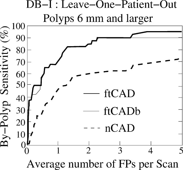
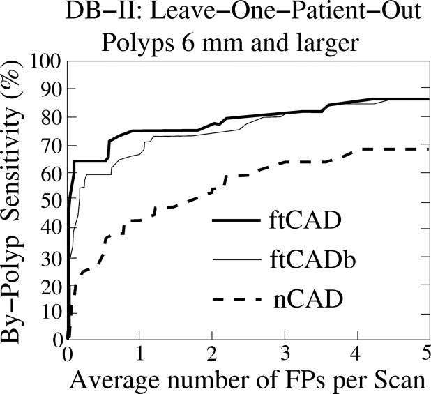
Pseudo-enhancement was minimized by use of an adaptive density correction (ADC) method. The presence of tagging was minimized by use of an adaptive density mapping (ADM) method. We also developed a new method for automated extraction of the colonic wall within air-filled and tagged regions. The ADC and ADM parameters were optimized by use of an anthropomorphic phantom. The CAD scheme was evaluated with 32+32 cases from two types of clinical ft CTC databases. The cases in database I had full cathartic cleansing and 40 polyps ≥6 mm, and the cases in database II had reduced cathartic cleansing and 44 polyps ≥6 mm. The by-polyp detection performance of the CAD scheme was evaluated by use of a leave-one-patient-out method with five features, and the results were compared with those of a conventional CAD scheme by use of free-response receiver operating characteristic curves.
Results
The CAD scheme detected 95% and 86% of the polyps ≥6 mm with 3.6 and 4.2 false positives per scan on average in databases I and II, respectively. For polyps ≥10 mm, the detection sensitivity was 94% in database I (with one missed hyperplastic polyp) and 100% in database II at the same false-positive rate. The detection sensitivity of the new CAD scheme was approximately 20% higher than that of the conventional CAD scheme.
Conclusions
The results show that the CAD scheme developed in this study resolves the technical challenges introduced by fecal tagging, is applicable to a variety of colon preparation regimens, and provides a performance superior to that of conventional CAD schemes.
Colorectal cancer is one of the three leading causes of cancer-related mortalities in the United States. Approximately 148,000 new cases and 55,000 deaths from colon cancer were estimated to occur in 2006 ( ). Screening can reduce colon cancer by facilitating the detection and removal of precancerous polyps. Colonoscopy is considered to have the highest diagnostic performance for screening of colon cancer, but it also has a high cost, risk of complications, and problems with patient compliance ( ).
Minimally invasive computed tomography colonography (CTC, also known as virtual colonoscopy ) can potentially yield a high diagnostic performance in the detection of clinically significant polyps ( ). As with colonoscopy, proper bowel preparation is necessary with CTC for confident detection of colorectal lesions. Residual materials and poor distension can reduce the sensitivity of CTC by obscuring polyps, and solid fecal materials can reduce the specificity of CTC by imitating polyps. The presence of fecal materials can be minimized by use of cathartic cleansing of the colon. However, cathartic cleansing is also a major barrier for patient compliance ( ).
Get Radiology Tree app to read full this article<
Get Radiology Tree app to read full this article<
Get Radiology Tree app to read full this article<
Get Radiology Tree app to read full this article<
Get Radiology Tree app to read full this article<
Get Radiology Tree app to read full this article<
Get Radiology Tree app to read full this article<
Get Radiology Tree app to read full this article<
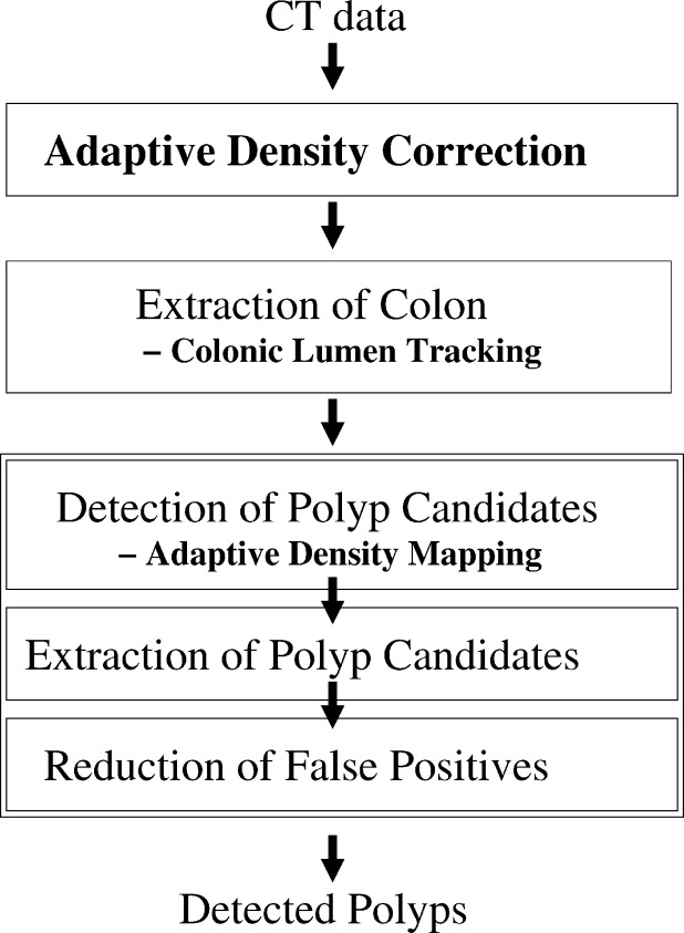
Materials and methods
Detection of Polyps
Get Radiology Tree app to read full this article<
Get Radiology Tree app to read full this article<
ADC Method
Get Radiology Tree app to read full this article<
Get Radiology Tree app to read full this article<
Get Radiology Tree app to read full this article<
υI(p)=υˆI(p)+υI(p)PEH, υ
I
(
p
)
=
υ
I
(
p
)
+
υ
I
(
p
)
PEH
,
where the additive term v I ( p ) PEH represents the effect of PEH at p . We estimate this term by modeling of the PEH as an iterative additive Gaussian effect as follows: Each voxel q with a high value of CT attenuation distributes residual pseudo-enhancement “energy” r 0 ( q ) to its neighboring voxels p according to a Gaussian function. This distributed energy is redistributed iteratively according to
rn(p)=∑qrn−1(q)2π√σ2(rn−1(q))exp(−12∣∣D(p,q)σ2(rn−1(q))∣∣2), r
n
(
p
)
=
∑
q
r
n
−
1
(
q
)
2
π
σ
2
(
r
n
−
1
(
q
)
)
exp
(
−
1
2
|
D
(
p
,
q
)
σ
2
(
r
n
−
1
(
q
)
)
|
2
)
,
where σ 2 ( r n−1 ( q )) represents the Gaussian spread of the distributed residual energy at q at iteration n − 1, and D ( p, q ) is the Euclidean distance between p and q . At each iteration, the residual energy that was distributed during previous iteration is redistributed according to Eq 2 . The iteration terminates when the redistributable energy becomes negligible. Then, the PEH is minimized by
υˆI(p)=υI(p)−υI(p)PEH≈υI(p)−∑Ni=0ri(p), υ
I
(
p
)
=
υ
I
(
p
)
−
υ
I
(
p
)
PEH
≈
υ
I
(
p
)
−
∑
i
=
0
N
r
i
(
p
)
,
where N is the number of iterations. An advantage of ADC is that it uses only the output data of a CT scanner, and thus it can be applied retrospectively to any CTC cases. After the application of the ADC, we can assume that CT attenuations ≤ t T ( t T ≈100 HU) represent untagged materials such as soft tissue and air, whereas higher CT attenuations indicate tagged materials.
Get Radiology Tree app to read full this article<
ADM Method
Get Radiology Tree app to read full this article<
Get Radiology Tree app to read full this article<
υ˙I=⎧⎩⎨⎪⎪⎪⎪υItT−(1000+tT)υI−tTtU−tT−1000υI≤tT,tT<υI<tU,υI≥tU. υ
˙
I
=
{
υ
I
υ
I
≤
t
T
,
t
T
−
(
1000
+
t
T
)
υ
I
−
t
T
t
U
−
t
T
t
T
<
υ
I
<
t
U
,
−
1000
υ
I
≥
t
U
.
Get Radiology Tree app to read full this article<
Get Radiology Tree app to read full this article<
Get Radiology Tree app to read full this article<
Get Radiology Tree app to read full this article<
Get Radiology Tree app to read full this article<
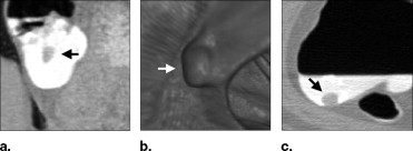
![Figure 3, (a) Left: A polyp located within the surface layer of tagged fluid (in the original computed tomography [CT] data). Middle: Effect of the application of Eq 4 . Right: The white region indicates the interface between air and tagged regions identified by the application of the gradient interface analysis method. (b) Left: The white region indicates an initially detected region (in the CT data interpolated to isotropic resolution). Right: The white region indicates the region of a polyp candidate extracted by conditional morphologic dilation (18).](https://storage.googleapis.com/dl.dentistrykey.com/clinical/FullyAutomatedThreeDimensionalDetectionofPolypsinFecalTaggingCTColonography/2_1s20S1076633206006738.jpg)
Get Radiology Tree app to read full this article<
Get Radiology Tree app to read full this article<
Get Radiology Tree app to read full this article<
υTI(n)(p)={10ifυI(p)≥n,otherwise. υ
T
I
(
n
)
(
p
)
=
{
1
if
υ
I
(
p
)
≥
n
,
0
otherwise
.
Let NT__I ( n ) ( p ) denote the negation of T__I ( n ) ( p ): if υ T__I ( n ) ( p ) = m ( m = 0,1), then υ NT__I ( n ) ( p ) = 1 – m . Let parameter t A denote the highest CT attenuation that represents air ( t A ≈ –700 HU). Then, the region of air is represented by A = NT I ( t A ), the tagged region is represented by T = T I ( t T ), and the soft-tissue region is represented by S = NT I ( t T ) ∩ T I ( t A ).
Get Radiology Tree app to read full this article<
Get Radiology Tree app to read full this article<
Get Radiology Tree app to read full this article<
Get Radiology Tree app to read full this article<
υ′′(p)={tT+700υI(p)ifυI(p)≥tT,otherwise. υ
″
(
p
)
=
{
t
T
+
700
if
υ
I
(
p
)
≥
t
T
,
υ
I
(
p
)
otherwise
.
Get Radiology Tree app to read full this article<
Get Radiology Tree app to read full this article<
A|T=T∇I’(t∇I’)∩T∇I′′(t∇I′′), A
|
T
=
T
∇
I
′
(
t
∇
I
′
)
∩
T
∇
I
″
(
t
∇
I
″
)
,
A|S=T∇I’(t∇I’)\T∇I′′(t∇I′′), A
|
S
=
T
∇
I
′
(
t
∇
I
′
)
\
T
∇
I
″
(
t
∇
I
″
)
,
S|T=T∇I′′(t∇I′′)\T∇I’(t∇I’). S
|
T
=
T
∇
I
″
(
t
∇
I
″
)
\
T
∇
I
′
(
t
∇
I
′
)
.
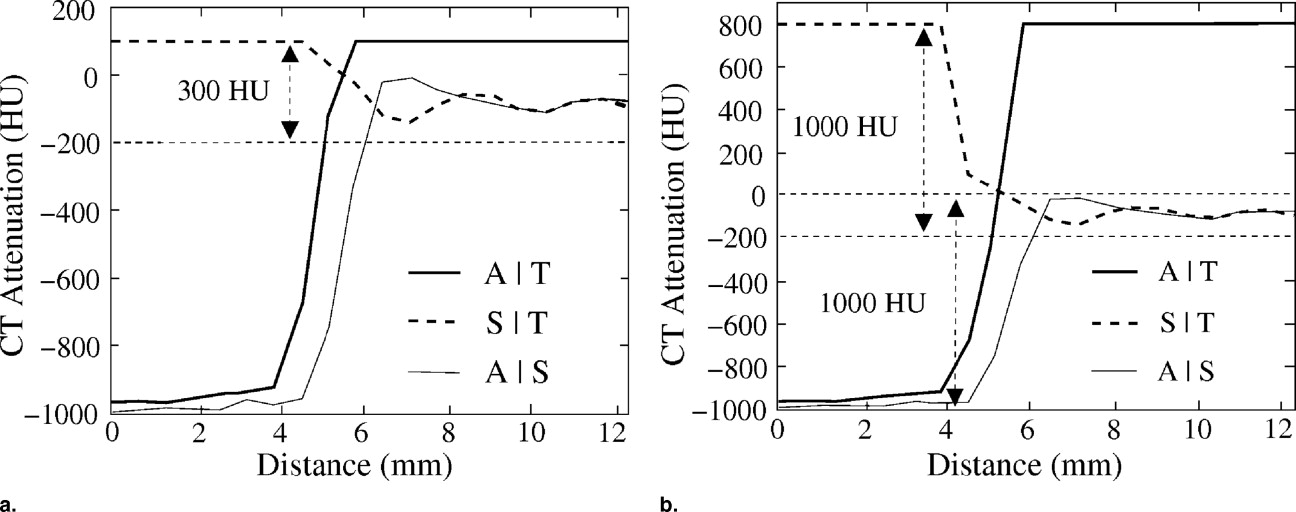
where t ∇ I ″ is set to exceed the highest contrast of the CT attenuation within the interfaces A ¦ S and S ¦ T . Thus we have obtained the region of the interface A ¦ T which is then excluded from the detection of polyp candidates as explained previously.
Get Radiology Tree app to read full this article<
Colonic Lumen Tracking Method
Get Radiology Tree app to read full this article<
Get Radiology Tree app to read full this article<
Get Radiology Tree app to read full this article<
D(Pe2r,Pe1k)+D(Pe2k,Pe1d)<D(Pe2r,Pe1l)+D(Pe2l,Pe1d) D
(
P
r
e
2
,
P
k
e
1
)
+
D
(
P
k
e
2
,
P
d
e
1
)
<
D
(
P
r
e
2
,
P
l
e
1
)
+
D
(
P
l
e
2
,
P
d
e
1
)
and
D(Pe2k,Pe1d)<D(Pe2r,Pe1d). D
(
P
k
e
2
,
P
d
e
1
)
<
D
(
P
r
e
2
,
P
d
e
1
)
.
Get Radiology Tree app to read full this article<
Get Radiology Tree app to read full this article<
Get Radiology Tree app to read full this article<
Get Radiology Tree app to read full this article<
Get Radiology Tree app to read full this article<
Get Radiology Tree app to read full this article<
Get Radiology Tree app to read full this article<
Parameter Estimation
Get Radiology Tree app to read full this article<
Get Radiology Tree app to read full this article<
Get Radiology Tree app to read full this article<
Get Radiology Tree app to read full this article<
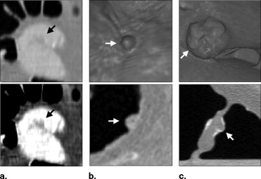
![Figure 5, Examples of line samples of 11 polyps that were covered by low-density (300 Hounsfield units [HU]; solid lines) and moderate-density (600 HU; dotted lines) tagging. The line samples were calculated after the application of the adaptive density correction method.](https://storage.googleapis.com/dl.dentistrykey.com/clinical/FullyAutomatedThreeDimensionalDetectionofPolypsinFecalTaggingCTColonography/5_1s20S1076633206006738.jpg)
Get Radiology Tree app to read full this article<
Get Radiology Tree app to read full this article<
Get Radiology Tree app to read full this article<
Evaluation of CAD Performance
Get Radiology Tree app to read full this article<
Get Radiology Tree app to read full this article<
Get Radiology Tree app to read full this article<
Get Radiology Tree app to read full this article<
Get Radiology Tree app to read full this article<
Get Radiology Tree app to read full this article<
Get Radiology Tree app to read full this article<
Results
Get Radiology Tree app to read full this article<
Get Radiology Tree app to read full this article<
Get Radiology Tree app to read full this article<
Get Radiology Tree app to read full this article<
Get Radiology Tree app to read full this article<
Get Radiology Tree app to read full this article<
Get Radiology Tree app to read full this article<
Get Radiology Tree app to read full this article<
Get Radiology Tree app to read full this article<
Get Radiology Tree app to read full this article<
Discussion
Get Radiology Tree app to read full this article<
Get Radiology Tree app to read full this article<
Get Radiology Tree app to read full this article<
Get Radiology Tree app to read full this article<
Get Radiology Tree app to read full this article<
Get Radiology Tree app to read full this article<
Conclusion
Get Radiology Tree app to read full this article<
Acknowledgments
Get Radiology Tree app to read full this article<
Get Radiology Tree app to read full this article<
References
1. Jemal A., Siegel R., Ward E., et. al.: Cancer statistics, 2006. CA Cancer J Clin 2006; 56: pp. 106-130.
2. Glick S.: Background and significance.Dachman A.Atlas of virtual colonoscopy.2003.Springer-VerlagNew York:pp. 5-9.
3. Pickhardt P., Choi J., Hwang I., et. al.: Computed tomographic virtual colonoscopy to screen for colorectal neoplasia in asymptomatic adults. N Engl J Med 2003; 349: pp. 2191-2200.
4. Gluecker T., Johnson C., Harmsen W., et. al.: Colorectal cancer screening with CT colonography, colonoscopy, and double-contrast barium enema examination: prospective assessment of patient perceptions and preferences. Radiology 2003; 227: pp. 378-384.
5. Lefere P., Gryspeerdt S., Dewyspelaere J., et. al.: Dietary fecal tagging as a cleansing method before CT colonography: initial results - polyp detection and patient acceptance. Radiology 2002; 24: pp. 393-403.
6. Zalis M., Perumpillichira J., Del Frate C., et. al.: CT colonography: digital subtraction bowel cleansing with mucosal reconstruction—initial observations. Radiology 2003; 226: pp. 911-917.
7. Iannaccone R., Laghi A., Magniapane F., et. al.: Computed tomographic colonography without cathartic preparation for the detection of colorectal polyps. Gastroenterology 2004; 127: pp. 1300-1311.
8. Lefere P., Gryspeerdt S.: 2006.SpringerBerlin, Germany
9. Yoshida H.: The future: computer-aided detection.Lefere P.Gryspeerdt S.2006.SpringerBerlin, Germany:pp. 137-152.
10. Yoshida H., Näppi J.: Three-dimensional computer-aided diagnosis scheme for detection of colonic polyps. IEEE Trans Med Imaging 2001; 20: pp. 1261-1274.
11. Yoshida H., Dachman A.: CAD techniques, challenges and controversies in computed tomographic colonography. Abdom Imaging 2004; 30: pp. 26-41.
12. Frimmel H., Näppi J., Yoshida H.: Centerline-based colon segmentation for CT colonography. Med Phys 2005; 32: pp. 2665-2672.
13. Summers R., Franaszek M., Miller M.: Computer-aided detection of polyps on oral contrast-enhanced CT colonography. AJR Am J Roentgenol 2005; 184: pp. 105-108.
14. Summers R., Yao J., Pickhardt P., et. al.: Computed tomographic virtual colonoscopy computer-aided polyp detection in a screening population. Gastroenterology 2005; 2005: pp. 1832-1844.
15. Zalis M., Yoshida H., Näppi J., et. al.: Evaluation of false positive detections in combined computer aided polyp detection and minimal preparation/digital subtraction CT colonography (CTC). Proc RSNA 2004; pp. 578.
16. Näppi J., Frimmel H., Dachman A., et. al.: A new high-performance CAD scheme for the detection of polyps in CT colonography.Fitzpatrick J.Sonka M.SPIE medical imaging 2004.2004.SPIE PressBellingham WA, USA:pp. 839-848.
17. Yoshida H., Näppi J., MacEneaney P., et. al.: Computer-aided diagnosis scheme for detection of polyps at CT colonography. Radiographics 2002; 22: pp. 963-979.
18. Näppi J., Yoshida H.: Feature-guided analysis for reduction of false positives in CAD of polyps for CT colonography. Med Phys 2003; 30: pp. 1592-1601.
19. Lefere P., Gryspeerdt S., Marrannes J., et. al.: CT colonography after fecal tagging with reduced cathartic cleansing and a reduced volume of barium. AJR Am J Roentgenol 2005; 184: pp. 1836-1842.
20. Näppi J., Okamura A., Frimmel H., et. al.: Region-based supine-prone correspondence for the reduction of false-positive CAD polyp candidates in CT colonography. Acad Radiol 2005; 12: pp. 695-707.
21. Kupinski M., Edwards D., Giger M., et. al.: Ideal observer approximation using Bayesian classification neural networks. IEEE Trans Med Imaging 2001; 20: pp. 886-899.
22. Näppi J., Yoshida H.: Automated detection of polyps in CT colonography: evaluation of volumetric features for reduction of false positives. Acad Radiol 2002; 9: pp. 386-397.
23. Näppi J, Yoshida H. Adaptive correction of CT attenuation for computer-aided detection of polyps in fecal-tagging CT colonography. Submitted.
24. Näppi J., Yoshida H.: Adaptive normalization of fecal-tagging CT colonography images for computer-aided detection of polyps. Int J Comp Assisted Radiol Surg 2006; 1: pp. 371-372.
25. Näppi J., MacEneaney P., Dachman A., et. al.: Knowledge-guided automated segmentation of colon for computer-aided detection of polyps in CT colonography. J Comput Assist Tomogr 2002; 26: pp. 493-504.
26. Frimmel H., Näppi J., Yoshida H.: Fast and robust computation of colon centerline in CT colonography. Med Phys 2004; 31: pp. 3046-3056.
27. Sethian J.: 1999.Cambridge University PressCambridge, MA
28. Zalis M., Perumpillichira J., Kim J., et. al.: Polyp size at CT colonography after electronic subtraction cleansing in an anthropomorphic colon phantom. Radiology 2005; 236: pp. 118-124.
29. Callstrom M., Johnson C., Fletcher J., et. al.: CT colonography without cathartic preparation: feasibility study. Radiology 2001; 219: pp. 693-698.
30. Bunch P., Hamilton J., Sanderson G., et. al.: A free-response approach to the measurement and characterization of radiographic-observer performance. J Appl Photogr Eng 1978; 4: pp. 166-171.
31. Metz C.: Evaluation of CAD methods.Doi K. et. al.Computer-Aided diagnosis in medical imaging.1999.Elsevier ScienceAmsterdam, The Netherlands:pp. 543-544.
32. Näppi J., Zalis M., Cai W., et. al.: CAD in minimal-preparation CT colonography: technical feasibility. Proc RSNA 2005; pp. 440.
33. Tourassi G., Floyd C.: The effect of data sampling on the performance evaluation of artificial neural networks in medical diagnosis. Med Decis Making 1997; 17: pp. 186-192.