
Rationale and Objectives
Derivation of diagnostically relevant parameters from first-pass myocardial perfusion magnetic resonance images involves the tedious and time-consuming manual segmentation of the myocardium in a large number of images. To reduce the manual interaction and expedite the perfusion analysis, we propose an automatic registration and segmentation method for the derivation of perfusion linked parameters.
Materials and Methods
A complete automation was accomplished by first registering misaligned images using a method based on independent component analysis, and then using the registered data to automatically segment the myocardium with active appearance models. We used 18 perfusion studies (100 images per study) for validation in which the automatically obtained (AO) contours were compared with expert drawn contours on the basis of point-to-curve error, Dice index, and relative perfusion upslope in the myocardium.
Results
Visual inspection revealed successful segmentation in 15 out of 18 studies. Comparison of the AO contours with expert drawn contours yielded 2.23 ± 0.53 mm and 0.91 ± 0.02 as point-to-curve error and Dice index, respectively. The average difference between manually and automatically obtained relative upslope parameters was found to be statistically insignificant ( P = .37). Moreover, the analysis time per slice was reduced from 20 minutes (manual) to 1.5 minutes (automatic).
Conclusion
We proposed an automatic method that significantly reduced the time required for analysis of first-pass cardiac magnetic resonance perfusion images. The robustness and accuracy of the proposed method were demonstrated by the high spatial correspondence and statistically insignificant difference in perfusion parameters, when AO contours were compared with expert drawn contours.
Contrast-enhanced magnetic resonance imaging (MRI) techniques, such as first-pass myocardial perfusion imaging, have become an important tool for diagnosis of ischemic heart disease. First-pass myocardial perfusion imaging involves the acquisition of MRI scans at the same phase during the first pass of contrast medium through heart in multiple cardiac cycles. This imaging process requires the acquisition of data over 45–60 seconds.
The main aim of perfusion imaging is the derivation of myocardial perfusion–linked parameters (eg, relative upslope), which requires tracking of regional myocardial intensity in all frames of a perfusion sequence as a function of time. Because the signal must be derived from the same myocardial region in successive frames to obtain accurate results, the perfusion assessment method must include correction measures for respiratory-induced motion of the myocardium. The most commonly used approach to assess myocardial perfusion involves the manual delineation of myocardium with epi- and endocardial contours by an expert (regarded as the gold standard). A typical perfusion sequence, as such, consists of 50–65 frames per slice; therefore, the task of manually segmenting the myocardium in each frame of the sequence is tedious and time consuming.
Get Radiology Tree app to read full this article<
Get Radiology Tree app to read full this article<
Get Radiology Tree app to read full this article<
Get Radiology Tree app to read full this article<
Get Radiology Tree app to read full this article<
Get Radiology Tree app to read full this article<
Background
ICA
Get Radiology Tree app to read full this article<
I=[g(x1,y1),g(x1,y2),g(x1,y3),……,g(xp,yq)]T I
=
[
g
(
x
1
,
y
1
)
,
g
(
x
1
,
y
2
)
,
g
(
x
1
,
y
3
)
,
…
…
,
g
(
x
p
,
y
q
)
]
T
and the complete perfusion sequence with n time points as:
X=[I1I2I3……In]T X
=
[
I
1
I
2
I
3
…
…
I
n
]
T
where, I t represents images at time points t = 1, 2, 3, ….., n . In the form of an ICA model, the observation space (a perfusion sequence) can be shown as:
X=X¯¯¯+WS X
=
X
¯
+
W
S
where S∈Rk×pq S
∈
ℜ
k
×
p
q consists of independent components and k is the number of retained components and pq represents the size of perfusion images. The matrix W∈Rn×k W
∈
ℜ
n
×
k in Equation 3 defines the weight coefficients representing the time-intensity variation of k component images and n is the number of frames per slice of the perfusion sequence.
Get Radiology Tree app to read full this article<
Get Radiology Tree app to read full this article<
AAM
Get Radiology Tree app to read full this article<
Model Building
Get Radiology Tree app to read full this article<
s=s¯+Qsbs s
=
s
¯
+
Q
s
b
s
Here, s is the mean shape, Q s consists of shape eigenvectors, and b s are the model deformation parameters.
Get Radiology Tree app to read full this article<
Get Radiology Tree app to read full this article<
Get Radiology Tree app to read full this article<
t=t¯+Qtbt t
=
t
¯
+
Q
t
b
t
where t¯ t
¯ is the mean texture and b t are the texture-related model deformation parameters. The parameter vectors b s and b t summarize the shape and texture of any sample from the training dataset. To recover the correlation between shapes and textures, we apply PCA on the concatenated vector:
bc=(Wsbsbt) b
c
=
(
W
s
b
s
b
t
)
which, based on Equations 4 and 5 , can also be written as:
bc=(WsQTs(s−s¯)QTt(t−t¯)) b
c
=
(
W
s
Q
s
T
(
s
−
s
¯
)
Q
t
T
(
t
−
t
¯
)
)
where W s is a diagonal matrix that consists of weight factors for the shape parameters. The PCA on the combined vector b c yields another model:
bc=Qaa b
c
=
Q
a
a
where Q a represent appearance eigenvectors and a represents appearance parameters that controls both the shape and the texture of the model. The use of simple linear algebra yields the expression for generating shape and texture instances in terms of combined model parameters, a :
s=s¯+QsW−1sQasa s
=
s
¯
+
Q
s
W
s
−
1
Q
a
s
a
t=t¯+QtQata t
=
t
¯
+
Q
t
Q
a
t
a
where,
Qa=(QasQat) Q
a
=
(
Q
a
s
Q
a
t
)
The model thus obtained gives a compact representation of the permissible variations in the appearance (shape and texture) as seen in the training set and allows the synthesis of a sample image for a given a by generating the shape-free texture image from the vector t and warping it using the control points described by s .
Get Radiology Tree app to read full this article<
Model Matching
Get Radiology Tree app to read full this article<
Get Radiology Tree app to read full this article<
Materials and methods
Data
AAM Training Data
Get Radiology Tree app to read full this article<
Perfusion Testing Data
Get Radiology Tree app to read full this article<
Ground Truth Contours
Get Radiology Tree app to read full this article<
Methods
Get Radiology Tree app to read full this article<

Get Radiology Tree app to read full this article<
ICA-based Registration
Get Radiology Tree app to read full this article<
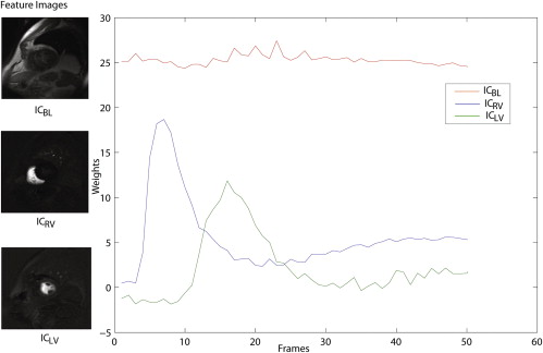
Computation and Labeling of Components
Get Radiology Tree app to read full this article<
Computation of the Region of Interest and Reference Image
Get Radiology Tree app to read full this article<
Get Radiology Tree app to read full this article<
Computation of the Displacements and Alignment of Frames
Get Radiology Tree app to read full this article<
Get Radiology Tree app to read full this article<
AAM-based Segmentation
Get Radiology Tree app to read full this article<
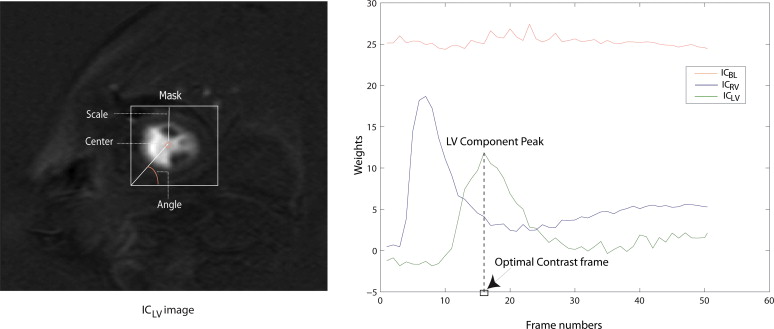
Derivation of Initialization Parameters
Get Radiology Tree app to read full this article<
Get Radiology Tree app to read full this article<
Selection of the Optimal Contrast Frame for Segmentation
Get Radiology Tree app to read full this article<
Validation Indices
Get Radiology Tree app to read full this article<
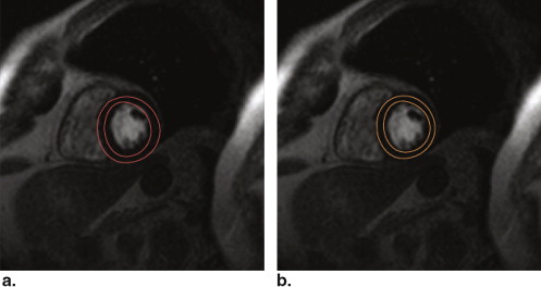
Spatial Correspondence
Get Radiology Tree app to read full this article<
Diceindex=2|P∩Q||P|+|Q| Dice
index
=
2
|
P
∩
Q
|
|
P
|
+
|
Q
|
where P and Q represent the areas corresponding to the overlapping contours.
Get Radiology Tree app to read full this article<
Myocardial Perfusion Analysis
Get Radiology Tree app to read full this article<
Statistical Analysis
Get Radiology Tree app to read full this article<
Implementation Details
Get Radiology Tree app to read full this article<
Results
Get Radiology Tree app to read full this article<

Get Radiology Tree app to read full this article<
Get Radiology Tree app to read full this article<

Get Radiology Tree app to read full this article<
Get Radiology Tree app to read full this article<
Table 1
A Comparison of Existing Methods with the Proposed Method Based on Point-to-curve Error (mm)
Methods Mean ± SD. (mm) Proposed method 2.23 ± 0.56 Stegmann et al 2.93 ± 0.84 Ólafsdóttir et al 3.44 ± 1.73
Table 2
Point-to-curve Distance Measurements (in mm) Obtained from the Comparison of Manual Contours from Observers A and B with Automatically Obtained (AO) Contours
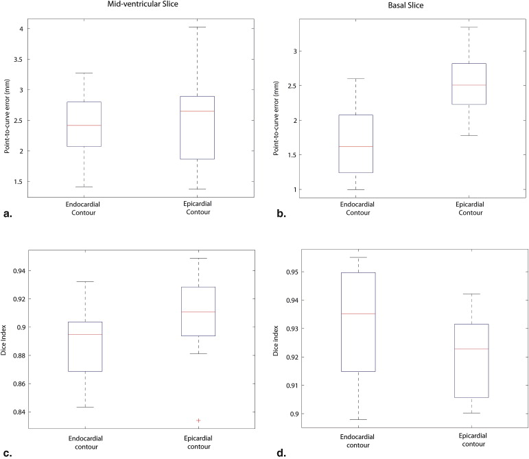
Contour comparisons Observer A vs. AO Observer B vs. AO Observer A vs. Observer B Contours Endocardial Epicardial Endocardial Epicardial Endocardial Epicardial Mid-ventricular slice 2.44 ± 0.53 2.55 ± 0.71 2.90 ± 0.68 3.08 ± 0.98 1.77 ± 0.57 2.08 ± 0.75 Basal slice 1.71 ± 0.53 2.55 ± 0.46 2.50 ± 0.62 2.51 ± 0.58 1.76 ± 0.49 2.02 ± 0.71
The last column shows inter-observer measurements. All values in the table are shown in the format: mean ± standard deviation.
Table 3
Dice Index Measurements Obtained from the Comparison of Manual Contours from Observers A and B with Automatically Obtained (AO) Contours
Contour comparisons Observer A vs. AO Observer B vs. AO Observer A vs. Observer B Contours Endocardial Epicardial Endocardial Epicardial Endocardial Epicardial Mid-ventricular slice 0.89 ± 0.02 0.91 ± 0.02 0.87 ± 0.03 0.88 ± 0.04 0.91 ± 0.03 0.93 ± 0.03 Basal slice 0.92 ± 0.02 0.93 ± 0.01 0.90 ± 0.02 0.92 ± 0.02 0.93 ± 0.02 0.93 ± 0.02
The last column shows inter-observer measurements. All values in the table are shown in the format: mean ± standard deviation.
Get Radiology Tree app to read full this article<
Get Radiology Tree app to read full this article<
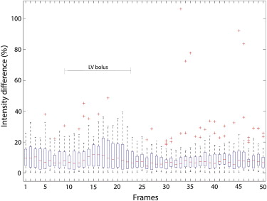

Table 4
Upslope Parameter Obtained using the Ground Truth and Automatically Obtained (AO) Contours for the Complete Dataset
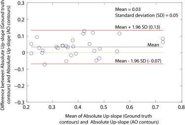
Parameter Ground Truth Contours AO Contours_P_ Value Relative upslope 0.11 ± 0.08 0.10 ± 0.08 .37 Absolute upslope 0.40 ± 0.13 0.38 ± 0.13 .26
Get Radiology Tree app to read full this article<
Get Radiology Tree app to read full this article<
Discussion
Get Radiology Tree app to read full this article<
Spatial Correspondence
Get Radiology Tree app to read full this article<
Myocardial Perfusion Analysis
Get Radiology Tree app to read full this article<
Limitations
Get Radiology Tree app to read full this article<
Future Perspectives
Get Radiology Tree app to read full this article<
Conclusion
Get Radiology Tree app to read full this article<
Acknowledgment
Get Radiology Tree app to read full this article<
References
1. Bidaut L., Vallée J.: Automated registration of dynamic MR images for the quantification of myocardial perfusion. J Magnet Res Imaging 2001; 13: pp. 648-655.
2. Breeuwer M., Spreeuwers L., Quist M.: Automatic quantitative analysis of cardiac MR perfusion images. Proc SPIE 2001; 4322: pp. 733.
3. Gupta S., Solaiyappan M., Beache G., et. al.: Fast method for correcting image misregistration due to organ motion in time-series MRI data. Magnet Res Med 2003; 49: pp. 506-514.
4. Bansal R., Funka-Lea G.: Integrated image registration for cardiac MR perfusion data. Lect Notes Computer Sci 2002; pp. 659-666.
5. Bracoud L., Vincent F., Pachai C., et. al.: Automatic registration of MR first-pass myocardial perfusion images. Lect Notes Computer Sci 2003; pp. 215-223.
6. Sun Y., Jolly M., Moura J.: Contrast-invariant registration of cardiac and renal MR perfusion images. Lect Notes Computer Sci 2004; pp. 903-910.
7. Gallippi C., Trahey G.: Automatic image registration for MR and ultrasound cardiac images. Lect Notes Computer Sci 2001; pp. 148-154.
8. Gao J., Ablitt N., Elkington A., et. al.: Deformation modelling based on PLSR for cardiac magnetic resonance perfusion imaging. Proc MICCAI 2002; 2488: pp. 612-619.
9. Discher A., Rougon N., Preteux F.: An unsupervised approach for measuring myocardial perfusion in MR image sequences. Proc SPIE 2005; 5916: pp. 126-137.
10. Rougon N., Discher A., Preteux F.: Region-driven statistical nonrigid registration: application to model- based segmentation and tracking of the heart in perfusion MRI. Proc SPIE 2005; 5916: pp. 148-159.
11. Dornier C., Ivancevic M., Thevenaz P., et. al.: Improvement in the quantification of myocardial perfusion using an automatic spline-based registration algorithm. J Magn Res Imaging 2003; 18: pp. 160-168.
12. Milles J., van der Geest R., Jerosch-Herold M., et. al.: Fully automated motion correction in first-pass myocardial perfusion MR image sequences. IEEE Trans Med Imaging 2008; 27: pp. 1611-1621.
13. Cootes T, Edwards G, Taylor C. Active appearance models. In 5th ECCV, volume 2, 1998.
14. Comon P.: Independent component analysis, a new concept?. Signal Proc 1994; 36: pp. 287-314.
15. Lee T.: Independent component analysis: theory and applications.1998.Kluwer Academic PublishersBoston, MA
16. Hyvarinen A., Oja E.: Independent component analysis: algorithms and applications. Neural Networks 2000; 13: pp. 411-430.
17. Carroll T., Haughton V., Rowley H., et. al.: Confounding effect of large vessels on MR perfusion images analyzed with independent component analysis. Am J Neuroradiol 2002; 23: pp. 1007.
18. Calhoun V., Adali T., Hansen L., et. al.: ICA of functional MRI data: an overview. In Proceedings of the International Workshop on Independent Component Analysis and Blind Signal Separation 2003; pp. 281-288.
19. Edwards G., Taylor C., Cootes T.: Interpreting face images using active appearance models. In 3rd International Conference on Automatic Face and Gesture Recognition 1998; pp. 300-305.
20. Mitchell S., Lelieveldt B., van der Geest R., et. al.: Multistage hybrid active appearance model matching: segmentation of left and right ventricles in cardiac MR images. IEEE Trans Med Imaging 2001; 20: pp. 415-423.
21. Bosch J., Mitchell S., Lelieveldt B., et. al.: Automatic segmentation of echocardiographic sequences by active appearance motion models. IEEE Trans Med Imaging 2002; 21: pp. 1374-1383.
22. Mitchell S., Bosch J., Lelieveldt B., et. al.: 3-D active appearance models: segmentation of cardiac MR and ultrasound images. IEEE Trans Med Imaging 2002; 21: pp. 1167-1178.
23. Stegmann M., Pedersen D.: Bi-temporal 3D active appearance models with applications to unsupervised ejection fraction estimation. Proc SPIE Med Image Proc 2005; 5747: pp. 336-350.
24. Stegmann M., Ólafsdóttir H., Larsson H.: Unsupervised motion-compensation of multi-slice cardiac perfusion MRI. Med Image Anal 2005; 9: pp. 394-410.
25. Gower J.: Generalized procrustes analysis. Psychometrika 1975; 40: pp. 33-51.
26. Bild D., Bluemke D., Burke G., et. al.: Multi-ethnic study of atherosclerosis: objectives and design. Am J Epidemiol 2002; 156: pp. 871.
27. van der Geest R., Reiber J.: Quantification in cardiac MRI. J Magnet Res Imaging 1999; 10: pp. 602-608.
28. Al-Saadi N., Gross M., Bornstedt A., et. al.: Comparison of various parameters for determining an index of myocardial perfusion reserve in detecting coronary stenosis with cardiovascular magnetic resonance tomography. Zeitschrift fur Kardiologie 2001; 90: pp. 824.
29. Jerosch-Herold M., Seethamraju R., Swingen C., et. al.: Analysis of myocardial perfusion MRI. J Magnet Res Imaging 2004; 19: pp. 758-770.
30. MATLAB (version 7.5).2007.The MathWorks IncNatick, MA
31. Ólafsdóttir H., Stegmann M., Ersbøll B., et. al.: A comparison of FFD-based nonrigid registration and AAMs applied to myocardial perfusion MRI. ProcSPIE 2006; 6144: pp. 614416.