Gain in Signal-to-Noise for First-Pass Contrast-Enhanced Abdominal MR Angiography at 3 Tesla Over Standard 1.5 Tesla Prediction with a Computer Model

Rationale and Objectives

To estimate the gain in signal-to-noise ratio (SNR) in first-pass contrast-enhanced (CE) abdominal magnetic resonance angiography (MRA) at 3.0 T compared with 1.5 T.

Materials and Methods

Three protocols were simulated using six contrast agents: gadopentetate dimeglumine (Magnevist, Berlex, Wayne, NJ), gadoteridol (Prohance, Bracco, Princeton, NJ), gadobenate dimeglumine (Multihance, Bracco, Princeton, NJ), gadodiamide (Omniscan, Amersham Health, Princeton, NJ), gadoversetamide (Optimark, Mallinckrodt, St. Louis, MO), and gadofosveset trisodium (MS-325, EPIX Medical, Cambridge, MA). Contrast concentrations were calculated for five abdominal vessels. Based on these data, the gain in SNR during CE abdominal MRA at 3.0 T over 1.5 T was estimated.

Results

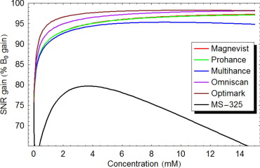
In these simulations, peak concentrations in all five target vessels were about 5 mM, 10 mM, and 0.7 mM for protocol 1, protocol 2, and protocol 3, respectively. A gain in SNR at 3 T over 1.5 T during CE abdominal MRA of at least 94% in all five target vessels could be achieved by applying protocol 1 or protocol 2, whereas protocol 3 provided a gain in SNR of 70%.

Conclusions

Although five of the contrast agents studied fulfill the expectation of providing approximately twice the SNR at 3.0 T versus 1.5 T during CE abdominal MRA, MS-325 offers a gain in SNR of 70% only.

Magnetic resonance (MR) imaging at 3 Tesla (T) has gained substantial interest in recent years resulting in a market share of approximately 10% (summer of 2006) of installed MR systems within the United States. In addition, with the latest introduction of dedicated receiver coils, most of the standard MR examinations have become possible at 3 T leading to a growing interest for routine clinical imaging of the abdomen and pelvis ( ).

The main argument for investing in 3.0 T MR imaging systems is the desire for a greater signal-to-noise ratio (SNR). As the intrinsic SNR increases proportional with the magnetic field strength, the theoretical gain in SNR is expected to be twofold when compared with a 1.5 T MR system ( ). However, tissue parameters such as the longitudinal relaxation time T1 and transverse relaxation time T2 also affect the intrinsic SNR. Unfortunately, T1 relaxation times increase with magnetic field strength and T2 relaxation times may slightly decrease with magnetic field strength, with both effects having a negative impact on the gain in SNR at higher magnetic field strengths ( ). In addition, field strength related changes of the relaxivity values of MR contrast agents (a measure of their “strength”) need to be considered as these values decrease with magnetic field strength ( ). All these effects combined raise the question how much contrast-enhanced (CE) MR imaging at 3 T will benefit from the higher field strength.

Get Radiology Tree app to read full this article<

Materials and methods

Background MR Physics

Get Radiology Tree app to read full this article<

SNR∝B0VvoxelTADC−−−−−√SSEQ S

∝

where B 0 is the main magnetic field strength, V voxel is the volume of each voxel without interpolation, T ADC is the total time that the analog to digital converter samples data for the image, and S SEQ is the sequence signal expression that describes the contrast and signal properties of the specific pulse sequence used.

Get Radiology Tree app to read full this article<

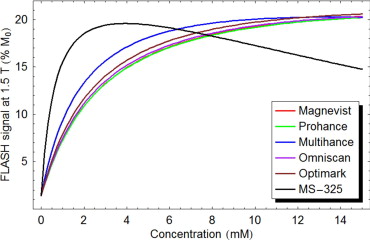
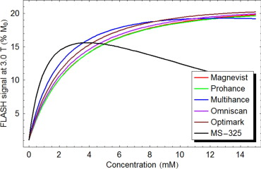
SFLASH=sin()e−TE/T2∗(1−e−TR/T1)1−cos()e−TR/T1 S

sin

⁡

(

)

−

(

−

)

−

cos

⁡

(

)

−

where θ is the flip angle, TR is the repetition time, TE is the echo time, and T1 and T2 \* are the longitudinal and transverse relaxation time, respectively. For short TR and reasonably large θ , the FLASH signal becomes strongly T1-weighted. Essentially only tissues with short T1 values are able to recover enough magnetization between repetitions to generate an appreciable signal.

Get Radiology Tree app to read full this article<

1T1(C)=1T1(0)+RC 1

(

)

(

)

where C is the in vivo MR contrast agent concentration, R is the relaxivity of the MR contrast agent, T1 (0) is the baseline T1 relaxation time, and T1 ( C ) is the T1 relaxation time after the administration of the MR contrast agent. The equation for T2 as a function of concentration is identical except that T1 is replaced by T2 . Equations 2 and 3 can be combined to obtain the FLASH signal as a function of the contrast agent concentration.

Get Radiology Tree app to read full this article<

MR Contrast Agents and Perfusion Model

Get Radiology Tree app to read full this article<

Table 1

Relaxivity Values R1 and R2 and Range of Various Magnetic Resonance Contrast Agents in Plasma at Two Different Field Strengths ⁎

1.5 T 3.0 T R1 (mM second) −1 R2 (mM second) −1 R1 (mM second) −1 R2 (mM second) −1 Gadopentetate dimeglumine (Magnevist) 4.1 (3.9–4.3) 4.6 (3.8–5.4) 3.7 (3.5–3.9) 5.2 (4.3–6.1) Gadoteridol (Prohance) 4.1 (3.9–4.3) 5.0 (4.2–5.8) 3.7 (3.5–3.9) 5.7 (4.8–6.6) Gadobenate dimeglumine (Multihance) 6.3 (6.0–6.6) 8.7 (7.8–9.6) 5.5 (5.2–5.8) 11 (10–12) Gadodiamide (Omniscan) 4.3 (4.4–4.8) 5.2 (4.2–6.2) 4.0 (3.8–4.2) 5.6 (4.7–6.5) Gadoversetamide (Optimark) 4.7 (4.4–5.0) 5.2 (4.3–6.1) 4.5 (4.2–4.8) 5.9 (5.0–6.8) Gadofosveset trisodium (MS-325) 19 (18–20) 34 (32–36) 9.9 (9.4–10.4) 60 (56–64)

R1 and R2 relaxivity values indicate the efficiency in shortening the longitudinal relaxation time T1 and transverse relaxation time T2, respectively.

Get Radiology Tree app to read full this article<

Table 2

Three Different Magnetic Resonance Contrast Agent Injection Protocols for a Human Adult With a Body Weight of 70 kg Based on Vendor Recommendations ( )

Injection Protocol Dosage (mmol/kg) Injection Volume (mL) Injection Rate (mL/second) 1 0.1 14 2 2 0.2 28 4 3 0.03 15 0.5

Get Radiology Tree app to read full this article<

Estimation of the Gain in SNR

Get Radiology Tree app to read full this article<

Results

Peak Arterial Concentrations

Get Radiology Tree app to read full this article<

Table 3

Peak Arterial Concentrations Predicted by a Computer Model in Five Different Abdominal Vessels Using Three Different Magnetic Resonance Contrast Agent Injection Protocols ( Table 2 ) for a Human Adult With a Body Weight of 70 kg ( )

Peak Arterial Concentration (mM) Upper Abdominal Aorta Celiac Trunk Proper Hepatic Artery Superior Mesenteric Artery Renal Artery Injection protocol 1 5.49 4.45 4.33 5.09 4.47 Injection protocol 2 10.97 8.90 8.67 10.19 8.95 Injection protocol 3 0.73 0.72 0.72 0.73 0.72

Get Radiology Tree app to read full this article<

Calculation of the Gain in SNR at 3.0 T Over 1.5 T

Get Radiology Tree app to read full this article<

Table 4

Effect of Various Magnetic Resonance Contrast Agents on the Longitudinal Relaxation Time T1 (in milliseconds) and Transverse Relaxation Time T2 (in milliseconds) of Blood at 1.5 T and 3 T Exemplified in the Renal Artery

Injection Protocol 1.5 Tesla 3.0 Tesla T1 Time T2 Time T1 Time T2 Time Blood without contrast agent NA 1441 290 1932 275 Blood and Magnevist 1 53 42 59 37 Blood and Prohance 1 53 39 59 34 Blood and Multihance 1 35 24 40 19 Blood and Omniscan 1 50 37 54 35 Blood and Optimark 1 46 37 48 33 Blood and MS-325 ⁎ 1 12 6 22 4 Blood and Magnevist 2 27 22 30 20 Blood and Prohance 2 27 21 30 18 Blood and Multihance 2 18 12 20 10 Blood and Omniscan 2 26 20 28 19 Blood and Optimark 2 23 20 25 18 Blood and MS-325 ⁎ 2 6 3 11 2 Blood and Magnevist ⁎ 3 274 148 314 135 Blood and Prohance ⁎ 3 274 142 314 129 Blood and Multihance ⁎ 3 191 103 223 87 Blood and Omniscan ⁎ 3 264 139 294 130 Blood and Optimark ⁎ 3 245 139 266 127 Blood and MS-325 3 70 36 131 21

Get Radiology Tree app to read full this article<

Table 5

Gain in Signal-to-Noise Ratio in Five Abdominal Arteries as a Percentage of B 0 Gain

Injection Protocol Upper Abdominal Aorta Celiac Artery Proper Hepatic Artery Superior Mesenteric Artery Renal Artery Magnevist 1 95.8 95.4 95.3 95.7 95.4 Prohance 1 95.8 95.3 95.3 95.6 95.3 Multihance 1 95.0 94.7 94.6 94.9 94.7 Omniscan 1 97.1 96.7 96.7 97.0 96.7 Optimark 1 98.0 97.8 97.8 97.9 97.8 MS-325 ⁎ 1 78.6 79.5 79.5 79.0 79.5 Magnevist 2 97.0 96.7 96.7 96.9 96.7 Prohance 2 96.9 96.6 96.6 96.8 96.7 Multihance 2 95.3 95.4 95.4 95.3 95.4 Omniscan 2 98.0 97.8 97.7 97.9 97.8 Optimark 2 98.3 98.3 98.3 98.3 98.3 MS-325 ⁎ 2 70.8 74.0 74.4 72.0 74.0 Magnevist ⁎ 3 89.9 89.8 89.8 89.9 89.8 Prohance ⁎ 3 89.9 89.8 89.8 89.9 89.8 Multihance ⁎ 3 89.3 89.3 89.3 89.3 89.3 Omniscan ⁎ 3 91.9 91.8 91.8 91.9 91.8 Optimark ⁎ 3 94.0 93.9 93.9 94.0 93.9 MS-325 3 69.8 69.7 69.7 69.8 69.7

Get Radiology Tree app to read full this article<

Discussion

Get Radiology Tree app to read full this article<

Gain in SNR

Get Radiology Tree app to read full this article<

Limitations

Get Radiology Tree app to read full this article<

Conclusion

Get Radiology Tree app to read full this article<

References

1. Hugg J., Rofsky N., Stokar S., et. al.: Clinical whole body MRI at 3.0 T—initial experience [abstract]. Proc Intl Mag Reson Med 2002; 10: pp. 569.
2. Sosna J., Rofsky N.M., Gaston S.M., et. al.: Determinations of prostate volume at 3-Tesla using an external phased array coil: comparison to pathologic specimens. Acad Radiol 2003; 10: pp. 846-853.
3. Katz-Brull R., Rofsky N.M., Lenkinski R.E.: Breathhold abdominal and thoracic proton MR spectroscopy at 3T. Magn Reson Med 2003; 50: pp. 461-467.
4. Gold G.E., Han E., Stainsby J., et. al.: Musculoskeletal MRI at 3.0 T: relaxation times and image contrast. Am J Roentgenol 2004; 183: pp. 343-351.
5. Gold G.E., Suh B., Sawyer-Glover A., et. al.: Musculoskeletal MRI at 3.0 T: initial clinical experience. Am J Roentgenol 2004; 183: pp. 1479-1486.
6. O’Regan D.P., Fitzgerald J., Allsop J., et. al.: A comparison of MR cholangiopancreatography at 1.5 and 3.0 Tesla. Br J Radiol 2005; 78: pp. 894-898.
7. Martin D.R., Friel H.T., Danrad R., et. al.: Approach to abdominal imaging at 1.5 Tesla and optimization at 3 Tesla. Magn Reson Imaging Clin N Am 2005; 13: pp. 241-254.
8. Morakkabati-Spitz N., Gieseke J., Kuhl C., et. al.: 3.0-T high-field magnetic resonance imaging of the female pelvis: preliminary experiences. Eur Radiol 2005; 15: pp. 639-644.
9. Merkle E.M., Dale B.M., Paulson E.K.: Abdominal MR imaging at 3.0 tesla. Magn Reson Imaging Clin N Am 2006; 14: pp. 17-26.
10. Merkle E.M., Haugan P.A., Thomas J., et. al.: MR cholangiography: 3.0 Tesla versus 1.5 Tesla—a pilot study. Am J Roentgenol 2006; 186: pp. 516-521.
11. Edelstein W.A., Glover G.H., Hardy C.J., et. al.: The intrinsic signal-to-noise ratio in NMR imaging. Magn Reson Med 1986; 3: pp. 604-618.
12. Bottomley P.A., Foster T.H., Argersinger R.E., et. al.: A review of normal tissue hydrogen NMR relaxation times and relaxation mechanisms from 1–100 MHz: dependence on tissue type, NMR frequency, temperature, species, excision, and age. Med Phys 1984; 11: pp. 425-448.
13. de Bazelaire C.M., Duhamel G.D., Rofsky N.M., et. al.: MR imaging relaxation times of abdominal and pelvic tissues measured in vivo at 3.0 T: preliminary results. Radiology 2004; 230: pp. 652-659.
14. Stanisz G.J., Odrobina E.E., Pun J., et. al.: T(1), T(2) relaxation and magnetization transfer in tissue at 3T. Magn Reson Med 2005; 54: pp. 507-512.
15. Rinck P.A., Muller R.N.: Field strength and dose dependence of contrast enhancement by gadolinium-based MR contrast agents. Eur Radiol 1999; 9: pp. 998-1004.
16. Weinmann H.J., Bauer H., Ebert W., et. al.: Comparative studies on the efficacy of MRI Contrast agents in MRA. Acad Radiol 2002; 9: pp. 135-136.
17. Trattnig S., Ba-Ssalamah A., Noebauer-Humann I.M., et. al.: MR contrast agent at high-field MRI (3 Tesla). Top Magn Reson Imaging 2003; 4: pp. 365-375.
18. Lee T., Stainsby J.A., Hong J., et. al.: Blood relaxation properties at 3T—effects of blood oxygen saturation. Proc Intl Mag Reson Med 2003; 11: pp. 131. (abstract)
19. Rohrer M., Bauer H., Mintorovitch J., et. al.: Comparison of magnetic properties of MRI contrast media solutions at different magnetic field strengths. Invest Radiol 2005; 40: pp. 715-724.
20. Trattnig S., Pinker K., Ba-Ssalamah A., et. al.: The optimal use of contrast agents at high field MRI. Eur Radiol 2006; 16: pp. 1280-1287.
21. Haacke E.M., Brown R.W., Thompson M.R.: 1999.John Wiley & SonsNew York, NY 340, 455
22. Bae K.T., Heiken J.P., Brink J.A.: Aortic and hepatic contrast medium enhancement at CT. Radiology 1998; 207: pp. 647-655.
23. Milnor W.R.: 1990.Oxford University PressOxford, UK
24. Wade O.L., Bishop J.M.: 1962.DavisPhiladelphia, Pa
25. Corot C., Violas X., Robert P., et. al.: Comparison of different types of blood pool agents (P792, MS325, USPIO) in a rabbit MR angiography-like protocol. Invest Radiol 2003; 38: pp. 311-319.
26. Hany T.F., Debatin J.F., Leung D.A., et. al.: Evaluation of the aortoiliac and renal arteries: comparison of breath-hold, contrast-enhanced, three-dimensional MR angiography with conventional catheter angiography. Radiology 1997; 204: pp. 357-362.
27. Hany T.F., Leung D.A., Pfammatter T., et. al.: Contrast-enhanced magnetic resonance angiography of the renal arteries. Invest Radiol 1998; 33: pp. 653-659.
28. Venkataraman S., Semelka R.C., Weeks S., et. al.: Assessment of aorto-iliac disease with magnetic resonance angiography using arterial phase 3-D gradient-echo and interstitial phase 2-D fat-suppressed spoiled gradient-echo sequences. J Magn Reson Imaging 2003; 17: pp. 43-53.
29. Prince M.R.: Contrast-enhanced MR angiography: theory and optimization. Magn Reson Imaging Clin N Am 1998; 6: pp. 257-267.
30. Schaefer P.J., Boudghene F.P., Brambs H.J., et. al.: Abdominal and iliac arterial stenoses: comparative double-blinded randomized study of diagnostic accuracy of 3D MR angiography with gadodiamide or gadopentetate dimeglumine. Radiology 2006; 238: pp. 827-840.
31. Rapp J.H., Wolff S.D., Quinn S.F., et. al.: Aortoiliac occlusive disease in patients with known or suspected peripheral vascular disease: safety and efficacy of gadofosveset-enhanced MR angiography—multicenter comparative phase III study. Radiology 2005; 236: pp. 71-78.
32. Prince M.R., Meaney J.F.M.: Expanding role of MR angiography in clinical practice. Eur Radiol 2006; 16: pp. B3-B8.
33. Edelman R.R., Salanitri G., Brand R., et. al.: Magnetic resonance imaging of the pancreas at 3.0 Tesla. Invest Radiol 2006; 41: pp. 175-180.
34. Riederer S.J., Bernstein M.A., Breen J.F., et. al.: Three-dimensional contrast-enhanced MR angiography with real-time fluoroscopic triggering: design specifications and technical reliability in 330 patient studies. Radiology 2000; 215: pp. 584-593.
35. Allkemper T., Heindel W., Koojman H., et. al.: Effect of field strengths on magnetic resonance angiography. Invest Radiol 2006; 41: pp. 97-104.
36. Runge V.M., Biswas J., Wintersperger B.J., et. al.: The efficacy of gadobenate dimeglumine (Gd-BOPTA) at 3 Tesla in brain magnetic resonance imaging. Invest Radiol 2006; 41: pp. 244-248.
37. Hartmann M., Wiethoff A.J., Hentrich H.R., et. al.: Initial imaging recommendations for Vasovist angiography. Eur Radiol 2006; 16: pp. B15-B23.
38. Nael K., Laub G., Finn J.P.: Three-dimensional contrast-enhanced MR angiography of the thoraco-abdominal vessels. Magn Reson Imaging Clin N Am 2005; 13: pp. 359-380.

Gain in Signal-to-Noise for First-Pass Contrast-Enhanced Abdominal MR Angiography at 3 Tesla Over Standard 1.5 Tesla Prediction with a Computer Model

Rationale and Objectives

Materials and Methods

Results

Conclusions

Materials and methods

Background MR Physics

MR Contrast Agents and Perfusion Model

Estimation of the Gain in SNR

Results

Peak Arterial Concentrations

Calculation of the Gain in SNR at 3.0 T Over 1.5 T

Discussion

Gain in SNR

Limitations

Conclusion

References

Further Reading

“Binary” and “Non-Binary” Detection Tasks Are Current Performance Measures Optimal?

2D or Not 2D That is the Question, But 3D is the Answer

3D and 2D Delayed-Enhancement Magnetic Resonance Imaging for Detection of Myocardial Infarction Preclinical and Clinical Results