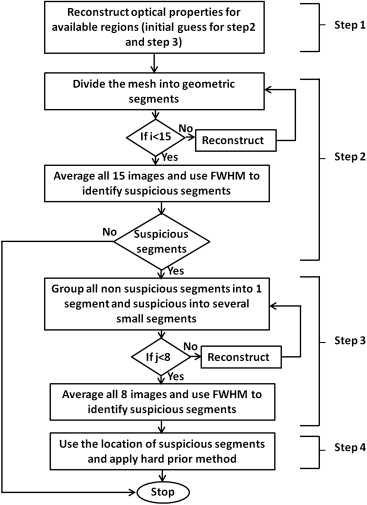
Hierarchical Clustering Method to Improve Transrectal Ultrasound-guided Diffuse Optical Tomography for Prostate Cancer Imaging

The inclusion of anatomical prior information in reconstruction algorithms can improve the quality of reconstructed images in near-infrared diffuse optical tomography (DOT). Prior literature on possible locations of human prostate cancer from transrectal ultrasound (TRUS), however, is limited and has led to biased reconstructed DOT images. In this work, we propose a hierarchical clustering method (HCM) to improve the accuracy of image reconstruction with limited prior information. HCM reconstructs DOT images in three steps: 1) to reconstruct the human prostate, 2) to divide the prostate region into geometric clusters to search for anomalies in finer clusters, 3) to continue the geometric clustering within anomalies for improved reconstruction. We demonstrated this hierarchical clustering method using computer simulations and laboratory phantom experiments. Computer simulations were performed using combined TRUS/DOT probe geometry with a multilayered model; experimental demonstration was performed with a single-layer tissue simulating phantom. In computer simulations, two hidden absorbers without prior location information were reconstructed with a recovery rate of 100% in their locations and 95% in their optical properties. In experiments, a hidden absorber without prior location information was reconstructed with a recovery rate of 100% in its location and 83% in its optical property.

Prostate cancer is one of the leading causes of cancer deaths in men in the United States . Conventional methods for diagnosing prostate cancer include the prostate-specific antigen (PSA) blood test and digital rectal examination (DRE). If the PSA level and/or DRE are suspicious, then in most cases the patient undergoes transrectal ultrasound (TRUS)–guided biopsy. This is because of the fact that the PSA level could be misleading. PSA can be expressed high because of benign prostatic hyperplasia. (BPH) . On the other hand, men with a low PSA level (<4.0 ng/ml) can still have prostate cancer . Despite recent advances in ultrasound, the grayscale-based ultrasound imaging has an accuracy of 50%–60% only; diagnosis accuracy can be even less in TRUS . Thus, TRUS has been used only for guiding a needle biopsy, not for the detection of prostate cancer. In recent years, researchers have made great advances in using magnetic resonance imaging (MRI) and magnetic resonance spectroscopy (MRS) to detect prostate cancer and/or to guide needle biopsy . Given MRI and MRS cost, bulkiness, requirement for body confinement, and limited accessibility to the general public, it is highly desirable to have a portable office-based imaging tool available to clinicians for an improved detection or screening of prostate cancer and for active surveillance to determine an optimal treatment time.

For the past two decades, diffuse optical tomography (DOT) with near-infrared (NIR) light has been a popular noninvasive imaging modality using nonionizing radiation to provide functional maps about the tissue under study. Because cancer tissues are more vasculature than the surrounding tissue, hemoglobin-based absorption in tumors provides optical contrast in DOT. When imaged at multiple wavelengths, DOT is capable of measuring chromophore concentrations such as oxyhemoglobin, deoxyhemoglobin, and water. Use of DOT for breast cancer detection and diagnosis has been extensively studied for nearly 20 years . However, investigations on detection of prostate cancer using DOT have been relatively limited compared to those done on breast cancer detection. A previous ex vivo study reported differences in water content between normal and cancer human prostate tissues. A recent review article provided a comprehensive summary of optical properties of human prostate cancer tissue at selective wavelengths. Specifically, several reports given in references show that light scattering of prostate cancer tissue is higher than that of normal prostate tissue. Transrectal DOT has been reported by several recent studies as a possible imaging tool for prostate cancer detection and diagnosis.

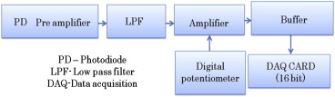
DOT instrumentation can be divided into three categories based on the principle of operation: 1) time-resolved systems , 2) frequency-domain systems , and 3) continuous wave (CW) systems . Measurements are made in transmission geometry, reflection geometry, or both. A time-resolved system relies on photon counting or gated imaging, which provides photons’ time of flight through the tissue. However, these systems are costly in comparison with CW systems. A frequency-domain system modulates laser light typically in the radio frequency range (100 MHz) and measures the amplitude and phase shift of the detected signal. A CW system is the simplest, fastest, and most cost-effective system in data collection; it can also be made at a video rate for imaging. However, CW systems measure only the intensity of reflected/transmitted light, so they cannot separate the absorption property from the scattering effect of the tissue .

For transrectal DOT to be able to provide excellent reconstructed images for prostate cancer detection, we have to acknowledge our obstacles to find appropriate solutions. One main obstacle is closely associated with the location of measurements: the human rectum, where we have a limited space (allowing a limited number of optodes to be implemented); furthermore, only reflectance geometry of DOT can be used. Given the nature of light scattering in tissues, DOT suffers from poor spatial resolution. Measurements taken using reflectance geometry do not normally achieve the excellent spatial resolution that is more commonly obtained in those taken by transmission geometry. One way to improve the spatial resolution is to couple DOT with other imaging techniques such as MRI and ultrasound. In particular, a combined TRUS and DOT probe for imaging prostate cancer has been studied previously , using the anatomical information from ultrasound to reduce the number of unknowns in the DOT image reconstruction. As shown by Xu et al. , each anatomical region was considered to be homogeneous; uniform optical properties were reconstructed in each respective region. Although the combined TRUS–DOT method improves accuracy of reconstructed DOT images, it relies highly on the ability of TRUS to locate the prostate cancer lesion. Given that TRUS has a low prostate cancer detection accuracy and that each region is assumed to be homogeneous, the reconstructed DOT images of prostate cancer could be erroneous.

To limit the dependency of DOT image reconstruction on TRUS sensitivity, we have developed a hybrid reconstruction technique by combining a piecewise cluster reconstruction approach with hard prior anatomy of prostate available from TRUS. Our method uses a hierarchical scheme of clustering, where we define a cluster as a group of nodes/voxels within a predefined volume. By using hierarchical clustering, a region of interest (ROI, ie, the prostate) can be transformed into a partially heterogeneous medium, within which we can search and further reconstruct potential cancer lesions. The inverse problem of DOT is solved in multiple steps by changing cluster sizes within the image domain. Multistep reconstruction in DOT has been reported earlier for breast cancer detection based on a frequency-domain study. It is understood according to Srinivasan et al. that the size and location of the absorber were partially or roughly estimated in the first step of reconstruction, after which more steps were used to further improve the quality of reconstructed images. In the TRUS–DOT scenario, however, a rough reconstruction of the first step is futile to effectively detect prostate cancer because of the multilayer tissue compositions, reflectance measurement geometry, limitation in the number of measurements, and particularly the inability of ultrasound to identify prostate cancer lesion or lesions. Thus, to improve the effectiveness and accuracy of prostate cancer imaging, we considered piecewise division of the image domain in DOT, assuming that the domain consists of disjoint subdomains with different optical properties.

Get Radiology Tree app to read full this article<

Methods

Forward and Inverse Methods in DOT

Get Radiology Tree app to read full this article<

−∇D(r→)∇Φ(r→,ω)+(μa(r→)+iω/c)Φ(r→,ω)=Qo(r→,ω) −

∇

(

→

)

∇

(

→

)

(

→

)

(

→

)

(

→

)

where Φ(r→,ω) Φ

(

→

) is the photon density at the position r→ r

→ , ω ω is the modulation frequency of light (in our study we use CW domain, so ω=0 ω

0 ), Qo(r→,ω) Q

(

→

) represents the isotropic source, c is the speed of light in the medium, and μa μ

a is the absorption coefficient; finally, D(r→) D

(

→

) is the optical diffusion coefficient which is defined as

D(r→)=1/3[μa(r→)+μ′s(r→)], D

(

→

)

[

(

→

)

’

(

→

)

]

where μ′s(r→) μ

’

(

→

) is the reduced scattering coefficient and is defined as μ′s(r→)=μs(r→)(1−g) μ

’

(

→

)

(

→

)

(

−

) . Here, μs(r→) μ

(

→

) is the scattering coefficient and g is the anisotropic factor. Equation can be solved using the finite element method (FEM) and applying Robin-type (type III or mixed) boundary condition to model the refractive index mismatch at the boundary.

Get Radiology Tree app to read full this article<

Ω=minD,μa{∥y−F(D,μa)∥2+λ∥(D,μa)−(D,μa0)∥2} Ω

min

{

‖

−

(

)

‖

(

)

−

(

)

‖

}

where y is a matrix to express all the measured data, F is the forward-calculation operator (or matrix) that generates diffusion-based light propagation responses, ∥∙∥2 ‖

•

‖

2 is the L2 norm, λ λ is the regularization parameter, and μ__a 0 is the initial estimate of light absorption coefficient. Note that the variables D , μ__a , and μ__a 0 are simplified notations for D(r→) D

(

→

) , μa(r→) μ

(

→

) , and μa0(r→) μ

(

→

) , respectively. By minimizing Equation , which is achieved by setting the first derivative of Equation with respect to μ__a as zero following Taylor series, and ignoring the second and higher order terms, we arrive at the updated equation:

(JTJ+λI)(δμa)=JT[y−F(μa)]+λ[(D,μa)−(D,μa0)] (

)

(

)

[

−

(

)

]

[

(

)

−

(

)

]

where J is the Jacobian matrix, I is the identity matrix, and δμ__a ( δμ__a = μ__a − μ__a 0 ) is a spatial distribution matrix of changes in μa μ

a with respect to the initial given value. Note that μ__a 0 is only the initial estimate at the first iteration. After the first iteration, μ__a 0 is basically the previous estimate. Now, Equation becomes Equation after we replace μ__a__− μ__a 0 by δμ__a ,

(JTJ+2λI)(δμa)=JT[y−F(μa)]. (

)

(

)

[

−

(

)

]

Get Radiology Tree app to read full this article<

Hierarchical Clustering

Get Radiology Tree app to read full this article<

J∗=JC, J

∗

where matrix C had the size of NN × NC (number of nodes × number of clusters). The elements of matrix C were given as follows:

C(i,j)={1ifi∈cj0else}, C

(

)

{

∈

}

where i marks the number of nodes and j marks the number of clusters. By the end of each iteration, the solution vector of δμ__a was mapped back to each node using Equation ,

δμa=C(δμ∗a) δ

(

∗

)

where δμ__a__\* is the vector with optical properties in respective geometric clusters solved from Equation . The function of matrix C is to transform the initial image domain into a new image domain where the inverse procedure is performed with cluster-based geometric structures. Matrix C is a mediator or operator that converts the regular geometry to and from cluster-based geometry for the reconstructed object. So, technically no inversion or transpose of C is directly involved.

Get Radiology Tree app to read full this article<

Simulation and experiment results

Transrectal DOT Image Reconstruction by HCM with Limited Prior Information

Get Radiology Tree app to read full this article<

Table 1

Comparison of Reconstructed μ a Values by Hierarchical Clustering Method with and without Prior Anatomical Information

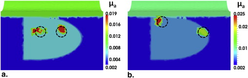
Tissue Type_μ__a_ (mm −1 ) Without Prior Information (%) With Prior Information (%) Periprostate 0.002 (100) 0.002 (100) Rectum wall 0.01 (100) 0.01 (100) Prostate 0.006 (100) 0.006 (100) Anomaly 0.019 (95) 0.02 (100)

Get Radiology Tree app to read full this article<

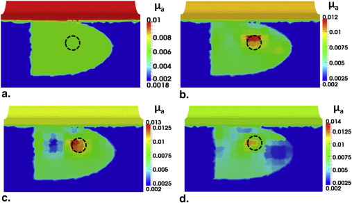
Investigation of HCM on Depth Sensitivity

Get Radiology Tree app to read full this article<

Table 2

Comparison of Reconstructed μ__a Value of the Target at Different Depths Using Hierarchical Clustering Method

Depth (cm) Target (mm −1 ) Reconstructed (mm −1 ) % Recovered of μ__a 1 0.02 0.019 95 2 0.02 0.019 95 3 0.02 — —

Get Radiology Tree app to read full this article<

Transrectal DOT Image Reconstruction by HCM with Two Absorbers

Get Radiology Tree app to read full this article<

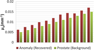
Investigation of HCM on Effects of Different Background (Prostate Region) Contrast

Get Radiology Tree app to read full this article<

Investigation of HCM on Effects of Different Noise Levels

Get Radiology Tree app to read full this article<

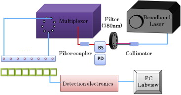
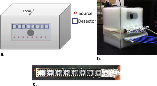
Experimental Demonstration

Get Radiology Tree app to read full this article<

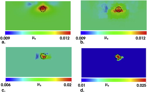
Table 3

Comparison of Reconstructed μ__a Value between Regular Diffuse Optical Method (DOT) Reconstruction and Hierarchical Clustering Method (HCM) for Experimental Data

Target (mm −1 ) Recovered (mm −1 ) Recovery Percentage (%) DOT reconstruction 0.03 0.0115 38.3 HCM 0.03 0.025 83.3

Get Radiology Tree app to read full this article<

Discussion

Investigation and Confirmation of HCM by Simulations and Phantom Experiments

Get Radiology Tree app to read full this article<

Potential Usefulness of HCM for Prostate Cancer Detection and Diagnosis

Get Radiology Tree app to read full this article<

Limitation of the Method and Future Work

Get Radiology Tree app to read full this article<

Conclusion

Get Radiology Tree app to read full this article<

Acknowledgment

Get Radiology Tree app to read full this article<

References

1. Siegel R., Naishadham D., Jemal A.: Cancer statistics, 2013. CA Cancer J Clin 2013; 63: pp. 11-30.
2. Diamandis E.P.: Prostate-specific antigen: its usefulness in clinical medicine. Trends Endocrinol Metab 1998; 9: pp. 310-316.
3. Monda J.M., Barry M.J., Oesterling J.E.: Prostate specific antigen cannot distinguish stage T1a (A1) prostate cancer from benign prostatic hyperplasia. J Urol 1994; 151: pp. 1291-1295.
4. Thompson I.M., Goodman P.J.: Prevalence of prostate cancer among men with a prostate-specific antigen level = 4.0 ng per milliliter. N Engl J Med 2004; 350: pp. 2239-2246.
5. Wijkstra H., Wink M.H., de la Rosette J.J.: Contrast specific imaging in the detection and localization of prostate cancer. World J Urol 2004; 22: pp. 346-350.
6. Kurhanewicz J., Vigneron D., Carroll P., et. al.: Multiparametric magnetic resonance imaging in prostate cancer: present and future. Curr Opin Urol 2008; 18: pp. 71-77.
7. deSouza N.M., Riches S.F., Vanas N.J., et. al.: Diffusion-weighted magnetic resonance imaging: a potential non-invasive marker of tumour aggressiveness in localized prostate cancer. Clin Radiol 2008; 63: pp. 774-782.
8. Tromberg B.J., Pogue B.W., Paulsen K.D., et. al.: Assessing the future of diffuse optical imaging technologies for breast cancer management. Med Phys 2008; 35: pp. 2443-2451.
9. Choe R., Konecky S.D., Corlu A., et. al.: Differentiation of benign and malignant breast tumors by in-vivo three-dimensional parallel-plate diffuse optical tomography. J Biomed Opt 2009; 14: pp. 024020.
10. Ali J.H., Wang W.B., Zevallos M., et. al.: Near infrared spectroscopy and imaging to probe differences in water content in normal and cancer human prostate tissues. Technol Cancer Res Treat 2004; 3: pp. 491-497.
11. Piao D., Bartels K.E., Jiang Z., et. al.: Alternative transrectal prostate imaging: a diffuse optical tomography method. IEEE J Sel Top Quantum Electron 2010; 10: pp. 519-531.
12. Svensson T., Andersson-Engels S., Einarsdóttír M., et. al.: In vivo optical characterization of human prostate tissue using near-infrared time-resolved spectroscopy. J Biomed Opt 2007; 12: pp. 014022.
13. Weersink R.A., Bogaards A., Gertner M., et. al.: Techniques for delivery and monitoring of TOOKAD (WST09)-mediated photodynamic therapy of the prostate: clinical experience and practicalities. J Photochem Photobiol B Biol 2005; 79: pp. 211-222.
14. Zhu T.C., Finlay J.C., Hahn S.M.: Determination of the distribution of light, optical properties, drug concentration, and tissue oxygenation in-vivo in human prostate during motexafin lutetium-mediated photodynamic therapy. J Photochem Photobiol B Biol 2005; 79: pp. 231-241.
15. Sharma V. A novel minimally invasive dual-modality fiber optic probe for prostate cancer detection. PhD dissertation, University of Texas at Arlington, 2011.
16. Jiang Z., Piao D., Xu G., et. al.: Trans-rectal ultrasound-coupled near-infrared optical tomography of the prostate, part II: experimental demonstration. Opt Express 2008; 16: pp. 17505-17520.
17. Wang K.K., Zhu T.C.: Reconstruction of in-vivo optical properties for human prostate using interstitial diffuse optical tomography. Opt Express 2009; 17: pp. 11665-11672.
18. Kavuri V.C., Liu H.: Hierarchical clustering method for improved prostate cancer imaging in diffuse optical tomography. Proc SPIE 2013; 8578: pp. 85781K.
19. Taroni P., Torricelli A., Spinelli L., et. al.: Time-resolved optical mammography between 637 and 985 nm: clinical study on the detection and identification of breast lesions. Phys Med Biol 2005; 50: pp. 2469-2488.
20. Pifferi A., Taroni P., Torricelli A., et. al.: Four-wavelength time-resolved optical mammography in the 680–980-nm range. Opt Lett 2003; 28: pp. 1138-1140.
21. Selb J., Joseph D.K., Boas D.A.: Time-gated optical system for depth-resolved functional brain imaging. J Biomed Opt 2006; 11: pp. 044008.
22. Pogue B., Testorf M., McBride T., et. al.: Instrumentation and design of a frequency-domain diffuse optical tomography imager for breast cancer detection. Opt Express 1997; 1: pp. 391-403.
23. Siegel A., Marota J.J., Boas D.: Design and evaluation of a continuous-wave diffuse optical tomography system. Opt Express 1999; 4: pp. 287-298.
24. Schmitz C.H., Klemer D.P., Hardin R., et. al.: Design and implementation of dynamic near-infrared optical tomographic imaging instrumentation for simultaneous dual-breast measurements. Appl Opt 2005; 44: pp. 2140-2153.
25. Arridge S.R., Lionheart W.R.: Nonuniqueness in diffusion-based optical tomography. Opt Lett 1998; 23: pp. 882-884.
26. Xu G., Piao D., Musgrove C.H., et. al.: Trans-rectal ultrasound-coupled near-infrared optical tomography of the prostate, part I: simulation. Opt Express 2008; 16: pp. 17484-17504.
27. Srinivasan S., Pogue B.W., Dehghani H.: Improved quantification of small objects in near-infrared diffuse optical tomography. J Biomed Opt 2004; 9: pp. 1161-1171.
28. Arridge S.R.: Optical tomography in medical imaging. Inverse problems 1999; 15: pp. 41.
29. Durduran T., Choe R., Baker W.B., et. al.: Diffuse optics for tissue monitoring and tomography. Rep Prog Phy 2010; 73: pp. 076701.
30. Haskell R.C., Svaasand L.O., Tsay T.T., et. al.: Boundary conditions for the diffusion equation in radiative transfer. J Opt Soc Am A Opt Image Sci Vis 1994; 11: pp. 2727-2741.
31. Dehghani H., Eames M.E., Yalavarthy P.K., et. al.: Near infrared optical tomography using NIRFAST: algorithm for numerical model and image reconstruction. Commun Numer Methods Eng 2008; 25: pp. 711-732.
32. Zacharopoulos A.D., Schweiger M., Kolehmainen V., et. al.: 3D shape based reconstruction of experimental data in diffuse optical tomography. Opt Express 2009; 17: pp. 18940-18956.
33. Kolehmainen V., Arridge S.R., Vauhkonen M., et. al.: Simultaneous reconstruction of internal tissue region boundaries and coefficients in optical diffusion tomography. Phys Med Biol 2000; 45: pp. 3267-3283.
34. Srinivasan S., Pogue B.W., Jiang S., et. al.: In vivo hemoglobin and water concentrations, oxygen saturation, and scattering estimates from near-infrared breast tomography using spectral reconstruction. Acad Radiol 2006; 13: pp. 195-202.

Hierarchical Clustering Method to Improve Transrectal Ultrasound-guided Diffuse Optical Tomography for Prostate Cancer Imaging

Methods

Forward and Inverse Methods in DOT

Hierarchical Clustering

Simulation and experiment results

Transrectal DOT Image Reconstruction by HCM with Limited Prior Information

Investigation of HCM on Depth Sensitivity

Transrectal DOT Image Reconstruction by HCM with Two Absorbers

Investigation of HCM on Effects of Different Background (Prostate Region) Contrast

Investigation of HCM on Effects of Different Noise Levels

Experimental Demonstration

Discussion

Investigation and Confirmation of HCM by Simulations and Phantom Experiments

Potential Usefulness of HCM for Prostate Cancer Detection and Diagnosis

Limitation of the Method and Future Work

Conclusion

Acknowledgment

References

Further Reading

Adaptable Near-Infrared Spectroscopy Fiber Array for Improved Coupling to Different Breast Sizes During Clinical MRI

Advances in Noninvasive Functional Imaging of Bone

Blood Flow Reduction in Breast Tissue due to Mammographic Compression