High Resolution Multidetector CT-Aided Tissue Analysis and Quantification of Lung Fibrosis

Rationale and Objectives

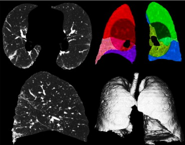
Volumetric high-resolution scans can be acquired of the lungs with multidetector CT (MDCT). Such scans have potential to facilitate useful visualization, characterization, and quantification of the extent of diffuse lung diseases, such as usual interstitial pneumonitis or idiopathic pulmonary fibrosis (UIP/IPF). There is a need to objectify, standardize, and improve the accuracy and repeatability of pulmonary disease characterization and quantification from such scans. This article presents a novel texture analysis approach toward classification and quantification of various pathologies present in lungs with UIP/IPF. The approach integrates a texture matching method with histogram feature analysis.

Materials and Methods

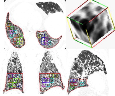
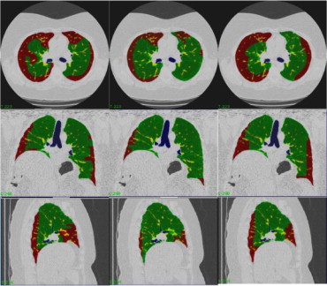
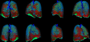
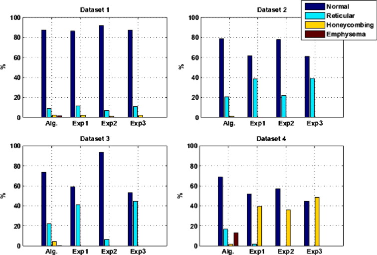
Patients with moderate UIP/IPF were scanned on a Lightspeed 8-detector GE CT scanner (140 kVp, 250 mAs). Images were reconstructed with 1.25-mm slice thickness in a high-frequency sparing algorithm (BONE) with 50% overlap and a 512 × 512 axial matrix, (0.625 mm 3 voxels). Eighteen scans were used in this study. Each dataset is preprocessed and includes segmentation of the lungs and the bronchovascular trees. Two types of analysis were performed, first an analysis of independent volume of interests (VOIs) and second an analysis of whole-lung datasets. 1) Fourteen of the 18 scans were used to create a database of independent 15 × 15 × 15 cubic voxel VOIs. The VOIs were selected by experts as having greater than 70% of the defined class. The database was composed of: honeycombing (number of VOIs 337), reticular (130), ground glass (148), normal (240), and emphysema (54). This database was used to develop our algorithm. Three progressively challenging classification experiments were designed to test our algorithm. All three experiments were performed using a 10-fold cross-validation method for error estimation. Experiment 1 consisted of a two-class discrimination: normal and abnormal. Experiment 2 consisted of a four-class discrimination: normal, reticular, honeycombing, and emphysema. Experiment 3 consisted of a five-class discrimination: normal, ground glass, reticular, honeycombing, and emphysema. 2) The remaining four scans were used to further test the algorithm on new data in the context of a whole lung analysis. Each of the four datasets was manually segmented by three experts. These datasets included normal, reticular and honeycombing regions and did not include ground glass or emphysema. The accuracy of the classification algorithm was then compared with results from experts.

Results

Independent VOIs: 1) two-class discrimination problem (sensitivity, specificity): normal versus abnormal (92.96%, 93.78%). 2) Four-class discrimination problem: normal (92%, 95%), reticular (86%, 87%), honeycombing (74%, 98%), and emphysema (93%, 98%). 3) Five-class discrimination problem: normal (92%, 95%), ground glass (75%, 89%), reticular (22%, 92%), honeycombing (74%, 91%), and emphysema (94%, 98%). Whole-lung datasets: 1) William’s index shows that algorithm classification of lungs agrees with the experts as well as the experts agree with themselves. 2) Student t -test between overlap measures of algorithm and expert (AE) and expert and expert (EE): normal ( t = −1.20, P = .230), Reticular ( t = −1.44, P = .155), Honeycombing ( t = −3.15, P = .003). 3) Lung volumes intraclass correlation: dataset 1 (ICC = 0.9984, F = 0.0007); dataset 2 (ICC = 0.9559, F = 0); dataset 3 (ICC = 0.8623, F= 0.0015); dataset 4 (ICC = 0.7807, F = 0.0136).

Conclusions

We have demonstrated that our novel method is computationally efficient and produces results comparable to expert radiologic judgment. It is effective in the classification of normal versus abnormal tissue and performs as well as the experts in distinguishing among typical pathologies present in lungs with UIP/IPF. The continuing development of quantitative metrics will improve quantification of disease and provide objective measures of disease progression.

Usual interstitial pneumonitis, or idiopathic pulmonary fibrosis (UIP/IPF), is a common type of interstitial pneumonia. This chronic, and typically progressive, pulmonary disease involves inflammation of the lung parenchyma, which results in ongoing fibrotic scar formation of the pulmonary interstitium and alveoli. The pathologic changes in lung morphology result in restrictive impairment of lung function. Restrictive diseases, such as UIP/IPF, result in decreased lung volumes, distortion of normal anatomy, and decreased parenchymal compliance. Thus there are significant deviations from normal lung function, the overall physiologic and mechanical effects of which can be demonstrated through pulmonary function testing, including reduction of total lung capacity, functional residual capacity, and lung compliance. To clarify the source of these functional abnormalities, characterize the disease process responsible for the changes, and visualize the extent of pulmonary involvement in diffuse lung disease, high-resolution computed tomography (HRCT) of the lungs is commonly used.

High-resolution imaging of the chest produces images that are less than 2-mm thick in the axial plane and that are optimized for visualization of the small anatomic structures of the secondary pulmonary lobule. Traditionally, technical limitations of CT scanners required that HRCT imaging protocols acquire noncontiguous thin slices (1 mm) every 10–20 mm. Thus only about 10% of the lung is imaged with resolution sufficient to visualize small pulmonary structures ( ). The improvements of computational and imaging technologies, including multidetector CT (MDCT), has made it possible to acquire isotropic three-dimensional higher resolution data of the entire chest in a single breathhold. An advantage of these MDCT scans, when properly acquired and reconstructed, is that volumetric high-resolution scans can be acquired of the lungs. Such scans allow for visualization, characterization, and quantification of the entire extent of diffuse lung diseases, such as UIP/IPF. The complex pathologic patterns that occur in UIP/IPF combined with the subjective nature of visual diagnosis and the labor-intensive task of 300 or more slices from apex to base of the lung results in a significant interobserver and intraobserver variability among radiologists attempting to classify and quantify these pathologic patterns.

Get Radiology Tree app to read full this article<

Materials and methods

Get Radiology Tree app to read full this article<

Data Preprocessing

Lung segmentation

Get Radiology Tree app to read full this article<

Bronchovascular segmentation

Get Radiology Tree app to read full this article<

Adaptive Binning of the Histogram

Get Radiology Tree app to read full this article<

C⎡⎣⎢⎢⎢i⎤⎦⎥⎥⎥⎡⎣⎢⎢⎢k⎤⎦⎥⎥⎥=min1≤i≤n,1≤j≤i⎧⎩⎨⎪⎪⎪⎪⎪⎪C⎡⎣⎢⎢⎢i⎤⎦⎥⎥⎥⎡⎣⎢⎢⎢k−1⎤⎦⎥⎥⎥,C⎡⎣⎢⎢⎢j⎤⎦⎥⎥⎥⎡⎣⎢⎢⎢k−1⎤⎦⎥⎥⎥+I⎡⎣⎢⎢⎢j+1⎤⎦⎥⎥⎥⎡⎣⎢⎢⎢i⎤⎦⎥⎥⎥⎫⎭⎬⎪⎪⎪⎪⎪⎪ C

[

]

[

]

min

⁡

≤

{

[

]

[

−

]

[

]

[

−

]

[

]

[

]

}

where C [ i ][ k − 1] is the minimum cost of splitting the histogram bins 0 to i into k − 1 clusters; similarly C [ j ][ k − 1] represents the minimum cost of splitting the histogram bins 0 to j into k − 1 bins, which is added to the cost of binning histogram bins j + 1 to i together.

Get Radiology Tree app to read full this article<

Signatures and the Canonical Signatures

Get Radiology Tree app to read full this article<

Sig={(μ1,w1),…,(μi,wi),…,(μK,wK)} S

{

(

)

…

(

)

…,

(

)

}

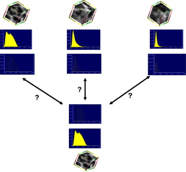
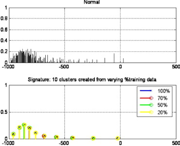
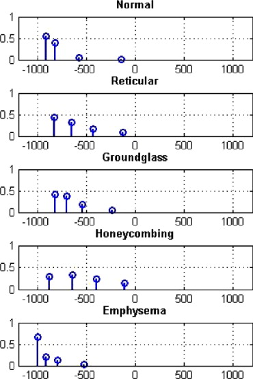
where μ i is the centroid of the cluster and w i is the weight of the cluster (the number of voxels in the cluster). The canonical signature for a class is computed by combining the signatures for each of the training VOIs and reclustering the distribution into K clusters. The creation of a canonical signature allows for a more computationally efficient way to match signatures instead of computing the distance between all training signatures and all test signatures. Each cluster centroid can be thought of as a texton, which is a cluster of intensity values representing some texture property ( ). Thus the signatures from each training image in each class are grouped or, in other words, all the textons are grouped and reclustered. Figure 3 shows the accumulated signatures in the top plot and the canonical signature created from various amounts of training data used in the bottom plot. Notice that an optimal clustering is achieved irrespective of the amount of training data used. The reclustering of all of the training signatures using the adaptive binning algorithm presented in the previous section maintains the integrity of the signatures; specifically the centroid location, the intracentroid distance, and the weight of the centroids. The clustering of the accumulated centroids results in a representative signature of K centroids. Figure 4 shows the representative canonical signatures computed in the development and testing of our algorithm for five classes.

Get Radiology Tree app to read full this article<

Similarity Metrics

Get Radiology Tree app to read full this article<

EMD(P,Q,F)=∑mi=1∑nj=1dijfij∑mi=1∑nj=1fij E

(



)

∑

such that, ∑jfij≤pj, ∑

≤

∑ifij≤qj, ∑

≤

∑i,jfij=min{∑ipi,∑jqj}, ∑

min

⁡

{

∑

and

fij≥0 f

≥

Get Radiology Tree app to read full this article<

Experimental Evaluation

Get Radiology Tree app to read full this article<

Data

Get Radiology Tree app to read full this article<

Training set: independent volumes of interest

Get Radiology Tree app to read full this article<

Testing set: whole-lung datasets

Get Radiology Tree app to read full this article<

Performance measures for analysis of classification of independent volumes of interest

Get Radiology Tree app to read full this article<

Sensitivityi=|Li||Ci| S

Specificityi=|Lj||Cj|,wherej=1,…,Nandj≠i S

where

…

≠

Get Radiology Tree app to read full this article<

Error=∑Ni=1∑Nj=1j≠i|Li||Cj| E

∑

≠

Get Radiology Tree app to read full this article<

Performance measures for analysis of classification of test lungs

Get Radiology Tree app to read full this article<

JC=X∩YX∪Y J

∩

∪

Get Radiology Tree app to read full this article<

VS=1−||X|−|Y|||X|+|Y| V

−

Get Radiology Tree app to read full this article<

WIj=(n−22)∑nj′=1,j′≠ja(Dj,Dj′)∑n−1j′=1,j′≠j∑nj′′>j′a(Dj′,Dj′′) W

(

−

)

∑

′

≠

(

′

)

∑

′

≠

−

∑

″

′

(

′

″

)

where a ( D j ,D j′ ) is a measure of similarity or agreement between raters j and j′ . We used two similarity measurements: JC and the volume similarity metric defined previously ( ). If the confidence interval (CI) of the Williams index for rater j includes 1, then it can be said that rater j agrees with the group as well as the members of the group agree with themselves. If the numerator and the denominator differ at the 100 α percent level, then the CI will not contain one.

Get Radiology Tree app to read full this article<

Results

Get Radiology Tree app to read full this article<

Independent Volumes of Interest

Get Radiology Tree app to read full this article<

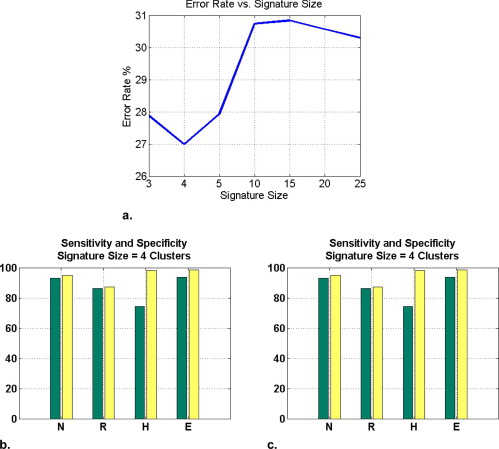
Table 1

Four-Class Confusion Matrix; Actual Class (Rows) versus Classified Class (Columns)

Normal Reticular Honeycombing Emphysema Normal 201 12 10 3 Reticular 6 109 66 0 Honeycombing 1 6 221 0 Emphysema 9 0 2 42

Table 2

Five-Class Confusion Matrix; Actual Class (Rows) versus Classified Class (Columns)

Normal Reticular Ground Glass Honeycombing Emphysema Normal 201 8 12 10 3 Reticular 5 26 14 35 0 Ground glass 1 44 95 31 0 Honeycombing 1 39 6 221 0 Emphysema 9 0 0 2 42

Get Radiology Tree app to read full this article<

Whole-Lung Datasets

Get Radiology Tree app to read full this article<

Table 3

Differences in Jaccard Overlap between the Average Algorithm/Expert (AE) Overlaps and the Expert/Expert (EE) Overlaps for Each Class Individually; The H 0 Hypothesis is μ 1 − μ 2 = 0

AE EE_t_ (62 Degree of freedom)P μAE, σAE μEE, σEE Normal 0.60, 0.27 0.68, 0.26 −1.20 .230 Reticular 0.18, 0.17 0.24, 0.21 −1.44 .155 Honeycombing 0.02, 0.06 0.19, 0.30 −3.15 .003 Emphysema 0, 0 0, 0 — —

Table 4

Hotelling T 2 Multivariate Test Comparing Algorithm/Expert with Expert-Expert Given All Four Classes

T 2 (3 Degree of freedom) F (29 Degree of freedom)P 26.15 8.15 .0004

Get Radiology Tree app to read full this article<

Discussion

Get Radiology Tree app to read full this article<

Normal

Get Radiology Tree app to read full this article<

Ground Glass

Get Radiology Tree app to read full this article<

Reticular

Get Radiology Tree app to read full this article<

Honeycombing

Get Radiology Tree app to read full this article<

Emphysema

Get Radiology Tree app to read full this article<

Conclusion

Get Radiology Tree app to read full this article<

References

1. Beigelman-Aubry C., Hill C., Guibal A., et. al.: Multi-detector row CT and postprocessing techniques in the assessment of diffuse lung disease. Radiographics 2005; 25: pp. 1639-1652.
2. Sutton R.N., Hall E.L.: Texture measures for automatic classification of pulmonary disease. IEEE Trans Computers 1972; 21: pp. 667-676.
3. Kruger R.P., Thompson W.B., Turner A.F.: Computer diagnosis of pneumoconiosis. IEEE Trans Sys Man Cybernetics 1974; 4: pp. 40-49.
4. Hall E.L., Crawford WO J., Roberts R.E.: Computer classification of pneumoconiosis from radiographs of coal workers. IEEE Trans Biomed Engineering 1975; 22: pp. 518-527.
5. Turner A.F., Kruger R.P., Thompson W.B.: Automated computer screening of chest radiographs for pneumoconiosis. Investig Radiol 1976; 11: pp. 258-266.
6. Tully R.J., Conners R.W., Harlow C.A., et. al.: Towards computer analysis of pulmonary infiltrites. Investig Radiol 1978; 13: pp. 298-305.
7. van Ginneken B., ter Haar Romeny B.M., Viergever M.A.: Computer-aided diagnosis in chest radiography: A survey. IEEE Trans Med Imaging 2001; 20: pp. 1228-1241.
8. Gilman M.J., Richard J., Laurens G., et. al.: CT attenuation values of lung density in sarcoidosis. J Comp Assisted Tomogr 1983; 7: pp. 407-410.
9. Müller N.L., Staples C.A., Miller R.R., et. al.: Density mask: an objective method to quantitate emphysema using computed tomography. Chest 1988; 94: pp. 782-787.
10. Rienmüller R.K., Behr J., Kalender W.A., et. al.: Standardized quantitative high resolution CT in lung disease. J Comp Assisted Tomogr 1991; 15: pp. 742-749.
11. Müller N.L., Coxson H.: Chronic obstructive pulmonary disease 4: Imaging the lungs in patients with chronic obstructive pulmonary disease. Thorax 2002; 57: pp. 982-985.
12. Goris M.L., Zhu H.J., Blankenberg F., et. al.: An automated approach to quantitative air trapping measurements in mild cystic fibrosis. Chest 2003; 123: pp. 1655-1663.
13. Hartley P.G., Galvin J.R., Hunninghake G.W., et. al.: High-resolution CT-derived measures of lung density are valid indexes of interstitial lung disease. J Appl Physiol 1994; 76: pp. 271-277.
14. Sluimer I., Schilham A., Prokop M., et. al.: Computer analysis of computed tomography scans of the lung: A survey. IEEE Trans Med Imaging 2006; 25: pp. 385-405.
15. Xu Y., McLennan G., Guo J., et. al.: MDCT-based 3-D texture classification of emphysema and early smoking related lung pathologies. IEEE Trans Medi Imaging 2006; 25: pp. 464-475.
16. Zaporozhan J., Ley S., Eberhardt R., et. al.: Paired inspiratory/expiratory volumetric thin-slice CT scan for emphysema analysis. Chest 2005; 128: pp. 3212-3220.
17. Mendonca P.R., Padfield D.R., Ross J.C., et. al.: Quantification of emphysema severity by histogram analysis of CT scans. MICCAI 2005; 8: pp. 738-744.
18. Rubner Y., Tomasi C., Guibas L.J.: The earth mover’s distance as a metric for image retrieval. Int J Comp Vision 2000; 40: pp. 99-121.
19. Varma M., Zisserman A.: A statistical approach to texture classification from single images. Int J Comp Vision 2005; 62: pp. 61-81.
20. Hu S., Hoffman E., Reinhardt J.: Automatic lung segmentation for accurate quantitation of volumetric X-ray CT images. IEEE Trans Med Imaging 2001; 20: pp. 490-498.
21. Aykac D., Hoffman E.A., McLennan G., et. al.: Segmentation and analysis of the human airway tree from 3D X-ray CT images. IEEE Trans Med Imaging 2003; 22: pp. 940-950.
22. Delorme S., Keller-Reichenbecher M.-A., Zuna I., et. al.: Usual interstitial pneumonia: Quantitative assessment of high-resolution computed tomography findings by computer-assisted texture-based image analysis. Investigative Radiology 1997; 32: pp. 566-574.
23. Hidenori S., Hoffman E.A., Sonka M.: Automated segmentation of pulmonary vascular tree from 3D CT images. Proc SPIE Med Imaging 2004; 5369: pp. 107-116.
24. Sato Y., Nakajima S., Atsumi H., et. al.: 3D multi-scale line filter for segmentation and visualization of curvilinear structures in medical images.1997.pp. 213-222.
25. Gonzalez R.C., Woods R.E., Eddins S.L.: 2004. Pearson Prentice Hall Upper Saddle River, NJ
26. Jain A., Murty M., Flynn P.: Data clustering: a review. ACM Comp Surv 1999; 31: pp. 264-323.
27. Knopps Z.F., Maintz J.B.A., Viergever M.A., et. al.: Normalized mutual information based registration using K-means clustering based histogram binning. Proc SPIE Med Imaging 2003; 5032: pp. 1072-1080.
28. Bellman R.: 1957.Princeton University PressPrinceton, NJ
29. Varma M., Zisserman A., IEEE Computer Society Conference on Computer Vision and Pattern Recognition: Texture classification: are filter banks necessary.2003.pp. 691.
30. Levina E., Bickel P., IEEE International Conference on Computer Vision: 2001.
31. Williams G.W.: Comparing the joint agreement of several raters with another rater. Biometrics 1976; 32: pp. 619-627.
32. Chalana V., Kim Y.: A methodology for evaluation of boundary detection algorithms on medical images. IEEE Trans Med Imaging 1997; 16: pp. 642-652.
33. Martin-Fernandez M., Bouix S., Ungar L., et. al.: Two methods for validating brain tissue classifiers. MICCAI 2005; 3749: pp. 515-522.
34. Hanley J.A., McNeil B.J.: The meaning and use of the area under a receiver operating characteristic (ROC) curve. Radiology 1982; 143: pp. 29-36.
35. Warfield S.K., Zou K.H., Wells W.M.: Simultaneous truth and performance level estimation (STAPLE). IEEE Trans Med Imaging 2004; 23: pp. 903-921.
36. Talmadge J., King E., Tooze J.A., et. al.: Predicting survival in idiopathic pulmonary fibrosis. Am J Resp Crit Care Med 2001; 164: pp. 1171-1181.
37. Wells A.U., Desai S.R., Rubens M.B., et. al.: Idiopathic pulmonary fibrosis: a composite physiologic index derived from disease extent observed by computed tomography. Am J Resp Crit Care Med 2006; 167: pp. 962-969.

High Resolution Multidetector CT-Aided Tissue Analysis and Quantification of Lung Fibrosis

Rationale and Objectives

Materials and Methods

Results

Conclusions

Materials and methods

Data Preprocessing

Lung segmentation

Bronchovascular segmentation

Adaptive Binning of the Histogram

Signatures and the Canonical Signatures

Similarity Metrics

Experimental Evaluation

Data

Training set: independent volumes of interest

Testing set: whole-lung datasets

Performance measures for analysis of classification of independent volumes of interest

Performance measures for analysis of classification of test lungs

Results

Independent Volumes of Interest

Whole-Lung Datasets

Discussion

Normal

Ground Glass

Reticular

Honeycombing

Emphysema

Conclusion

References

Further Reading

“Binary” and “Non-Binary” Detection Tasks Are Current Performance Measures Optimal?

2D or Not 2D That is the Question, But 3D is the Answer

3D and 2D Delayed-Enhancement Magnetic Resonance Imaging for Detection of Myocardial Infarction Preclinical and Clinical Results