
Rationale and Objectives
Accurate image segmentation for breast lesions is a critical step in computer-aided diagnosis systems. The objective of this study was to develop a robust method for the automatic segmentation of breast masses on mammograms to extract feasible features for computer-aided diagnosis systems.
Materials and Methods
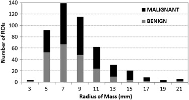
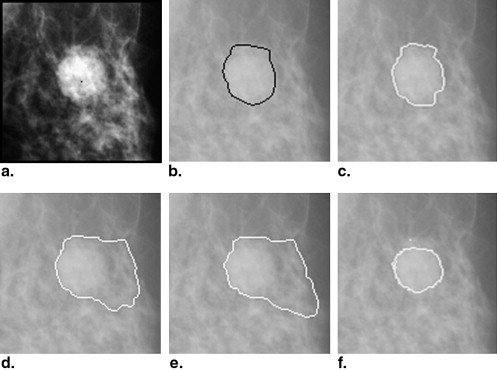
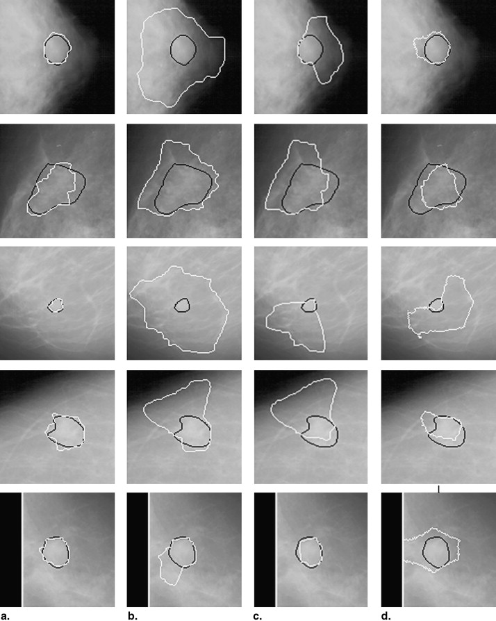
The data set used in this study consisted of 483 regions of interest extracted from 328 patients. A hybrid method for segmenting breast masses was proposed on the basis of the template-matching and dynamic programming techniques. First, a template-matching technique was used to locate and obtain the rough region of masses. Then, on the basis of this rough region, a local cost function for dynamic programming was defined. Finally, the optimal contour was derived by applying dynamic programming as an optimization technique. The performance of this proposed segmentation method was evaluated using area-based and boundary distance–based similarity measures based on radiologists’ manually marked annotations. A comparison with three different segmentation algorithms on the data set was provided.
Results
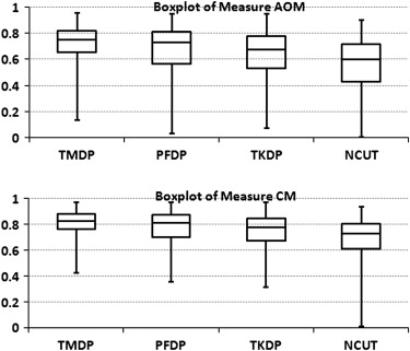
The mean overlap percentage for our proposed hybrid method was 0.727 ± 0.127, whereas those for Timp and Karssemeijer’s dynamic programming method, Song et al’s plane-fitting and dynamic programming method, and the normalized cut segmentation method were 0.657 ± 0.216, 0.636 ± 0.190, and 0.562 ± 0.199, respectively. All P values for the measure distribution of our proposed method and the other three algorithms were <.001.
Conclusions
A hybrid method based on the template-matching and dynamic programming techniques was proposed to segment breast masses on mammograms. Evaluation results indicate that the proposed segmentation method can improve the accuracy of mass segmentation compared to three other algorithms. The proposed segmentation method shows better performance and has great potential in improving the accuracy of computer-aided diagnosis systems in interpreting mammograms.
Computer-aided diagnosis (CAD) systems for mammography play a vital role in early cancer diagnosis and thus aid in reducing the mortality rate of breast cancer . Over the past decades, many CAD systems have been developed . Because their contours are crucial in the characterization of masses , an automatic segmentation of masses is one of the most important steps in any CAD system. An accurate contour of a lesion should be close to the actual mass boundary to provide feasible features and enable distinct discrimination between masses and regions corresponding to normal tissues. Mass boundaries are usually embedded and hidden in varying densities of parenchymal structures. Those boundaries are usually obscured, irregular, and of low contrast, so mass segmentation is a challenging task. In recent years, many approaches have been proposed for mass segmentation on mammograms. Those segmentation approaches can be divided into two main categories: region based and edge based .
The goal of region-based method is the detection of regions (connected sets of pixels) that satisfy certain predefined homogeneity criteria . Zheng et al and Park et al applied a multilayer topographic region-growing algorithm to segment and define the mass region boundary. The seed pixel is to choose the pixel with minimum gray value inside the initially labeled region, and the growing is adaptive on the basis of the computation of region contrast. A similar multilayer topographic region-growing algorithm and its effectiveness in defining mass boundary contours were reported by Eltonsy et al . Rather than focusing on local features and their consistencies in the image data, the normalized cut (NCUT) method proposed by Shi and Malik aims to extract the global impression of an image and solves image segmentation as a graph partitioning problem.
Get Radiology Tree app to read full this article<
Get Radiology Tree app to read full this article<
Get Radiology Tree app to read full this article<
Materials and methods
Data Set
Get Radiology Tree app to read full this article<
Get Radiology Tree app to read full this article<
Get Radiology Tree app to read full this article<
Image Segmentation Performance Evaluation
Get Radiology Tree app to read full this article<
AOM=Aseg∩AgsA∪segAgs, AOM
=
A
seg
∩
A
gs
A
∪
seg
A
gs
,
where A seg denotes the area of automatically segmented mass, and A gs is the corresponding ground-truth area provided by radiologists’ manually delineated outlines. The second quantitative measure is a combined measure (CM) of the undersegmentation, the oversegmentation, and the AOM:
CM=[AOM+(1−Ags−AsegAgs)+(1−Aseg−AgsAseg)]/3. CM
=
[
AOM
+
(
1
−
A
gs
−
A
seg
A
gs
)
+
(
1
−
A
seg
−
A
gs
A
seg
)
]
/
3
.
In addition, two distance measures, the average minimum Euclidean distance (AMED) and the Hausdorff distance (HD), were considered in this study. Given two contours, A = { a 1 , a 2 ,…, a m } and B = { b 1 , b 2 ,…, b n }, to be compared, the AMED( A , B ) and the HD( A , B ) are respectively defined as
AMED(A,B)=max[1m∑mi=1d(ai,B),1n∑nj=1d(bj,A)], AMED
(
A
,
B
)
=
max
[
1
m
∑
i
=
1
m
d
(
a
i
,
B
)
,
1
n
∑
j
=
1
n
d
(
b
j
,
A
)
]
,
HD(A,B)=max[maxi∈{1,…,m}{d(ai,B)},maxj∈{1,…,n}{d(bj,A)}], HD
(
A
,
B
)
=
max
[
max
i
∈
{
1
,
…
,
m
}
{
d
(
a
i
,
B
)
}
,
max
j
∈
{
1
,
…
,
n
}
{
d
(
b
j
,
A
)
}
]
,
where d(ai,B)=minj∈{1,…,m}∥ai−bj∥ d
(
a
i
,
B
)
=
min
j
∈
{
1
,
…
,
m
}
‖
a
i
−
b
j
‖ is the distance from a i to the closest point on the contour B .
Get Radiology Tree app to read full this article<
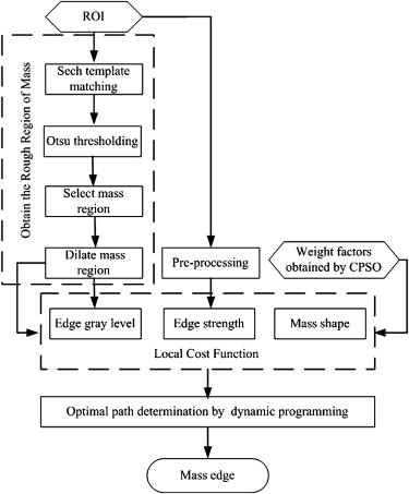
The Framework of Segmentation Algorithms
Get Radiology Tree app to read full this article<
Get Radiology Tree app to read full this article<
Step 1: Locate and Obtain the Rough Regions of Masses by Sech Template Matching
Get Radiology Tree app to read full this article<
T(x,y)=2exp(β×x2+y2√)+exp(−β×x2+y2√). T
(
x
,
y
)
=
2
exp
(
β
×
x
2
+
y
2
)
+
exp
(
−
β
×
x
2
+
y
2
)
.
Let the center of the template image to be the origin point and T ( x , y ) the gray level of the template image at the position ( x , y ). The rate of change on the gray level in the template from the center to the boundary is controlled by parameter β. Let L be the number of pixels on every edge of the template image, and then the template obtains the maximum value of gray level at the center and the minimum value at L /2 away. The values for the parameters L and β were set to 35 and 0.08, respectively, in this study. Let I denote the ROI image and μ T and μ I ( x , y ) denote the average gray level of the template image and the subregion of the ROI image (with the same size to template image) around the center point ( x , y ), respectively. The overlapping region of the template and the ROI image was represented by x ′ = 0… L − 1, y ′ = 0… L − 1. The similarity measure between the template and the ROI image at point ( i , j ), which indicates the similarity between them, is defined as
R(x,y)=1σT×σI∑x′,y′[T′(x′,y′)×I′(x+x′,y+y′)] R
(
x
,
y
)
=
1
σ
T
×
σ
I
∑
x
′
,
y
′
[
T
′
(
x
′
,
y
′
)
×
I
′
(
x
+
x
′
,
y
+
y
′
)
]
where
T′(x′,y′)=T(x′,y′)−μT, T
′
(
x
′
,
y
′
)
=
T
(
x
′
,
y
′
)
−
μ
T
,
I′(x+x′,y+y′)=I(x+x′,y+y′)−μI(x,y), I
′
(
x
+
x
′
,
y
+
y
′
)
=
I
(
x
+
x
′
,
y
+
y
′
)
−
μ
I
(
x
,
y
)
,
σT=∑x′,y′T′(x′,y′)2−−−−−−−−−−−−−√ σ
T
=
∑
x
′
,
y
′
T
′
(
x
′
,
y
′
)
2
and
σI=∑x′,y′I′(x+x′,y+y′)2−−−−−−−−−−−−−−−−−−−√, σ
I
=
∑
x
′
,
y
′
I
′
(
x
+
x
′
,
y
+
y
′
)
2
,
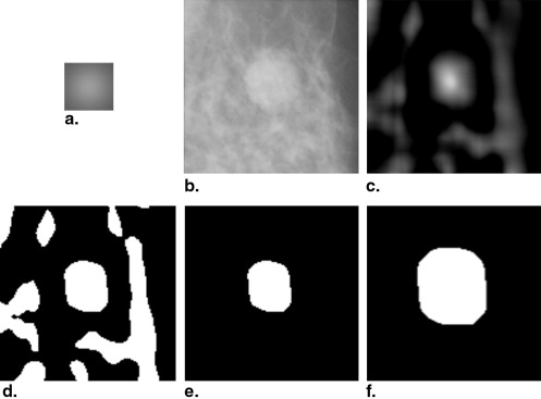
The value of the similarity measure of every pixel in the ROI image forms a correlation image (with the same size to the ROI image; see Fig 3 c). To locate and obtain the rough region of the mass, the correlation image is thresholded using the Otsu thresholding technique. In other words, pixels with correlation values below the threshold will not be considered as the candidates of masses (see Fig 3 d). In mammography CAD systems, the ROIs are located near the center of the suspicious masses (which are obtained by the detection method). To minimize the oversegmentation of the mass, we remove all other isolated regions, and only the nearest one from the center of the ROI is retained as the rough region of the mass (see Fig 3 e). The rough region will be used to define the local cost function of the dynamic programming algorithm in the follow-up step. For the case that the multiple regions are overlapped or connected, as long as the actual mass region is within the rough region, it will not have a great impact on the segmentation result. On the other hand, to ensure the rough region contains all the boundary points and minimize the undersegmentation of the mass, the rough region is dilated with a disk structuring element with a radius of 10 pixels (see Fig 3 f). The contour of the dilated rough region is considered as the preliminary contour of the mass.
Get Radiology Tree app to read full this article<
Get Radiology Tree app to read full this article<
Step 2: Construction of Local Cost Function
Get Radiology Tree app to read full this article<
Get Radiology Tree app to read full this article<
C(r,)={wSS(r,)+wGG(r,)+wII(r,)Mifr≤rˆ()else, C
(
r
,
)
=
{
w
S
S
(
r
,
)
+
w
G
G
(
r
,
)
+
w
I
I
(
r
,
)
if
r
≤
r
ˆ
(
)
M
else
,
where S , G , and I represent the shape feature, edge strength (gradient), and deviation from expected gray level (intensity), respectively. Parameter rˆ() r
ˆ
(
) represents the “radius” estimated for column by the rough region of masses obtained in step 1. Parameters w G , w D , and w I are the corresponding weights. When the point r () inside the rough region, that is, r≤rˆ() r
≤
r
ˆ
(
) , the local cost value is calculated by the sum of these three components. Otherwise, the local cost value is penalized by a large value M , which is implemented as the maximum integer number in the experiments.
Get Radiology Tree app to read full this article<
Step 2.1: Calculation of Components of the Local Cost Function
Get Radiology Tree app to read full this article<
S(r,)={d(r,)−dmindmax−dmin∞ifd(r,)≤drelse, S
(
r
,
)
=
{
d
(
r
,
)
−
d
min
d
max
−
d
min
if
d
(
r
,
)
≤
d
r
∞
else
,
where
d(r,)=r2+r2−1−2rr−1cos(1)−−−−−−−−−−−−−−−−−−−√ d
(
r
,
)
=
r
2
+
r
−
1
2
−
2
r
r
−
1
cos
(
1
)
and r and r −1 are the radii of columns and ( − 1), respectively. Parameters d max and d min are the maximum and minimum distance, respectively, between two points on adjacent columns. Empirical parameter dr is defined (the value used in this study was set to 3) to prevent sharp changes of the radii in two adjacent columns.
Get Radiology Tree app to read full this article<
Get Radiology Tree app to read full this article<
G(r,)=gmax−g(r,)gmax, G
(
r
,
)
=
g
max
−
g
(
r
,
)
g
max
,
where g ( r , ) is the magnitude of radial gradient at point ( r , ), and g max is the 99th percentile of the gradient values measured in the ROI.
Get Radiology Tree app to read full this article<
Get Radiology Tree app to read full this article<
I(r,)=∣∣i(r,)−(αi¯mass+(1−α)i¯background)∣∣−−−−−−−−−−−−−−−−−−−−−−−−−−−−−−√, I
(
r
,
)
=
|
i
(
r
,
)
−
(
α
i
¯
mass
+
(
1
−
α
)
i
¯
background
)
|
,
where i ( r , ) is the gray level value (intensity) of the pixel located at ( r , ), and i¯mass i
¯
mass and i¯background i
¯
background are the mean gray levels inside and outside, respectively, of the rough region of the mass. The value of parameter α should be <0.5 to ensure the edge is located toward the background level. The specific value of the parameter α in this study was 0.2. To represent the component of deviation from expected gray level in local cost function, the value of I ( r , ) is normalized:
I(r,)=Imax−I(r,)Imax−Imin, I
(
r
,
)
=
I
max
−
I
(
r
,
)
I
max
−
I
min
,
where I max and I min are the maximum and the minimum intensity of the candidate points, respectively. The value of I ( r , ) ranges from 0 to 1, with 0 indicating a high possibility to be the edge and 1 a low possibility.
Get Radiology Tree app to read full this article<
Step 2.2: The Optimization of Weights Using CPSO
Get Radiology Tree app to read full this article<
Get Radiology Tree app to read full this article<
Get Radiology Tree app to read full this article<
vt+1i=wvti+c1r1(pti−xti)+c2r2(ptg−xti) v
i
t
+
1
=
w
v
i
t
+
c
1
r
1
(
p
i
t
−
x
i
t
)
+
c
2
r
2
(
p
g
t
−
x
i
t
)
and
xt+1i=xti+vt+1i, x
i
t
+
1
=
x
i
t
+
v
i
t
+
1
,
where t denotes the iteration number, c 1 and c 2 are learning factors, and r 1 and r 2 are random numbers uniformly distributed in the range of [0,1]. The so-called inertia weight w is used to control the impact of the previous history of velocities on the current one.
Get Radiology Tree app to read full this article<
Get Radiology Tree app to read full this article<
Get Radiology Tree app to read full this article<
Step 3: Delineation of Lesion Outlines Using Dynamic Programming Technique
Get Radiology Tree app to read full this article<
CC(r,+1)=⎧⎩⎨⎪⎪⎪⎪∞C(r,0)min−3≤l≤3CC(r−l,)+C(r,+1)if(r<3orr>60)and≥0if(3≤r≤60)and=0otherwise, C
C
(
r
,
+
1
)
=
{
∞
C
(
r
,
0
)
min
−
3
≤
l
≤
3
C
C
(
r
−
l
,
)
+
C
(
r
,
+
1
)
i
f
(
r
<
3
or
r
60
)
and
≥
0
i
f
(
3
≤
r
≤
60
)
and
=
0
otherwise
,
where CC is the cumulative cost, C is the local cost function, and l indicates a direction of movement from column to column + 1. The path with lowest total cost can be found by tracing the path from one of the pixels in the last column to one of the pixels in the first column.
Get Radiology Tree app to read full this article<
Get Radiology Tree app to read full this article<
Results
Get Radiology Tree app to read full this article<
Get Radiology Tree app to read full this article<
Get Radiology Tree app to read full this article<
Table 1
Descriptive Statistics of the Distribution of Four Segmentation Measures for Each of Four Segmentation Methods
Method Minimum 0.25 Quartile Mean Median 0.75 Quartile Maximum Descriptive statistics of AOM TMDP 0.135 0.655 0.727 0.749 0.824 0.955 PFDP 0.030 0.564 0.658 0.728 0.813 0.951 TKDP 0.073 0.531 0.636 0.678 0.779 0.950 NCUT 0.001 0.429 0.562 0.601 0.714 0.902 Descriptive statistics of CM TMDP 0.423 0.758 0.810 0.826 0.879 0.970 PFDP 0.353 0.699 0.765 0.813 0.871 0.967 TKDP 0.311 0.670 0.744 0.777 0.845 0.967 NCUT 0.007 0.610 0.694 0.726 0.806 0.934 Descriptive statistics of AMED (mm) TMDP 0.440 1.127 1.762 1.503 2.103 11.451 PFDP 0.498 1.270 3.130 1.809 3.265 16.930 TKDP 0.500 1.314 2.879 1.913 3.286 14.067 NCUT 0.213 1.360 2.818 2.077 3.483 11.496 Descriptive statistics of HD (mm) TMDP 1.563 4.132 5.719 5.227 7.231 18.401 PFDP 1.658 4.469 7.660 6.473 9.652 22.024 TKDP 1.589 4.395 7.347 6.024 9.594 21.621 NCUT 1.603 4.431 7.058 6.482 9.247 21.649
AMED, average minimum Euclidean distance; AOM, area overlap measure; CM, combined method; HD, Hausdorff distance; NCUT, normalized cut method; PFDP, plane-fitting and dynamic programming; TKDP, Timp and Karssemeijer’s dynamic programming method; TMDP, template-matching and dynamic programming method.
Get Radiology Tree app to read full this article<
Get Radiology Tree app to read full this article<
Table 2
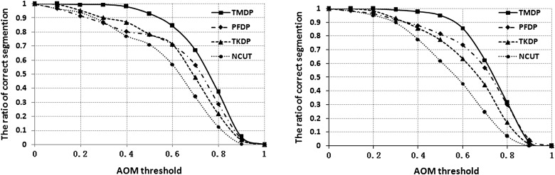
A Summary of the Numbers of Mass Correctly Segmented at Various Threshold Levels for the Two Segmentation Measures AOM and CM
Method ≥0.9 ≥0.8 ≥0.7 ≥0.6 ≥0.5 ≥0.4 ≥0.3 ≥0.2 ≥0.1 ≥0 Number of nodules with AOM in the corresponding sections TMDP 19 165 312 412 455 473 480 482 483 483 PFDP 21 143 274 350 387 408 433 455 472 483 TKDP 10 93 221 324 376 416 443 469 482 483 NCUT 1 46 139 244 319 374 428 457 472 483 Number of nodules with CM in the corresponding sections TMDP 69 297 429 470 480 483 483 483 483 483 PFDP 58 258 361 405 438 472 483 483 483 483 TKDP 44 204 345 404 445 473 483 483 483 483 NCUT 11 128 276 368 430 462 473 478 480 483
AOM, area overlap measure; CM, combined method; HD, Hausdorff distance; NCUT, normalized cut method; PFDP, plane-fitting and dynamic programming; TKDP, Timp and Karssemeijer’s dynamic programming method; TMDP, template-matching and dynamic pro-gramming method.
Get Radiology Tree app to read full this article<
Get Radiology Tree app to read full this article<
Table 3
The Mean Values of AOM and AMED for Five Mass Margin Types
Method Circumscribed Ill Defined Microlobulated Obscured Spiculated Mean values of AOM TMDP 0.727 0.722 0.777 0.762 0.692 PFDP 0.629 0.672 0.695 0.658 0.641 TKDP 0.634 0.630 0.707 0.673 0.580 NCUT 0.619 0.518 0.631 0.592 0.503 Mean values of AMED (mm) TMDP 1.695 1.675 1.606 1.606 2.114 PFDP 3.469 2.534 3.036 3.273 3.574 TKDP 2.942 2.528 2.397 2.510 3.761 NCUT 2.371 2.776 2.584 2.938 3.410
AMED, average minimum Euclidean distance; AOM, area overlap measure; NCUT, normalized cut method; PFDP, plane-fitting and dynamic programming; TKDP, Timp and Karssemeijer’s dynamic programming method; TMDP, template-matching and dynamic programming method.
Get Radiology Tree app to read full this article<
Discussion
Get Radiology Tree app to read full this article<
Get Radiology Tree app to read full this article<
Get Radiology Tree app to read full this article<
Get Radiology Tree app to read full this article<
Conclusions
Get Radiology Tree app to read full this article<
Get Radiology Tree app to read full this article<
References
1. Rangayyan R.M., Ayres F.J., Leo Desautels J.E.: A review of computer-aided diagnosis of breast cancer: toward the detection of subtle signs. J Franklin Inst 2007; 344: pp. 312-348.
2. Morton M.J., Whaley D.H., Brandt K.R., et. al.: Screening mammograms: interpretation with computer-aided detection—prospective evaluation. Radiology 2006; 239: pp. 375-383.
3. Masotti M., Lanconelli N., Campanini R.: Computer-aided mass detection in mammography: false positive reduction via gray-scale invariant ranklet texture features. Med Phys 2009; 36: pp. 311-316.
4. Eltonsy N.H., Tourassi G.D., Elmaghraby A.S.: A concentric morphology model for the detection of masses in mammography. IEEE Trans Med Imaging 2007; 26: pp. 880-889.
5. Varela C., Timp S., Karssemeijer N.: Use of border information in the classification of mammographic masses. Phys Med Biol 2006; 51: pp. 425-442.
6. Timp S., Karssemeijer N.: A new 2D segmentation method based on dynamic programming applied to computer aided detection in mammography. Med Phys 2004; 31: pp. 958-971.
7. Haris K., Efstratiadis S.N., Maglaveras N., et. al.: Hybrid image segmentation using watersheds and fast region merging. IEEE Trans Image Proc 1998; 7: pp. 1684-1699.
8. Zheng B., Chang Y.H., Gur D.: Computerized detection of masses in digitized mammograms using single-image segmentation and a multilayer topographic feature analysis. Acad Radiol 1995; 2: pp. 959-966.
9. Park S.C., Pu J., Zheng B.: Improving performance of computer-aided detection scheme by combining results from two machine learning classifiers. Acad Radiol 2009; 16: pp. 266-274.
10. Shi J., Malik J.: Normalized cuts and image segmentation. IEEE Trans Patt Anal Machine Intell 2000; 22: pp. 888-905.
11. Yuan Y., Giger M.L., Li H., et. al.: A dual-stage method for lesion segmentation on digital mammograms. Med Phys 2007; 34: pp. 4180-4193.
12. Amini A., Weymouth T.E., Jain R.C.: Using dynamic programming for solving variational problems in vision. IEEE Trans Patt Anal Machine Intell 1990; 12: pp. 855-867.
13. Nuyts J., Suetens P., Oosterlinck A., et. al.: Delineation of ECT images using global constraints and dynamic programming. IEEE Trans Med Imaging 1991; 10: pp. 489-498.
14. Aoyama M., Li Q., Katsuragawa S., et. al.: Computerized scheme for determination of the likelihood measure of malignancy for pulmonary nodules on low-dose CT images. Med Phys 2003; 30: pp. 387-394.
15. Wang J., Engelmann R., Li Q.: Segmentation of pulmonary nodules in three-dimensional CT images by use of a spiral-scanning technique. Med Phys 2007; 34: pp. 4678-4689.
16. Wang Q., Song E., Jin R., et. al.: Segmentation of lung nodules in computed tomography images using dynamic programming and multidirection fusion techniques. Acad Radiol 2009; 16: pp. 678-688.
17. Fracheboud J., de Koning H.J., Beemsterboer P.M.M., et. al.: Nation-wide breast cancer screening in the Netherlands: results of initial and subsequent screening 1990-1995. J Cancer 1998; 75: pp. 694-698.
18. Suckling J, Parker J, Dance D, et al. The Mammographic Image Analysis Society Digital Mammogram Database. Available at: http://peipa.essex.ac.uk/info/mias.html . Accessed August 6, 2010.
19. Heath M., Bowyer K., Kopans D., et. al.: Current status of the digital database for screening mammography.Karssemeijer N.Thijssen M.Hendriks J. et. al.Digital mammography.1998.KluwerBoston:pp. 457-460.
20. Rojas Domínguez A., Nandi A.K.: Improved dynamic-programming-based algorithms for segmentation of masses in mammograms. Med Phys 2007; 34: pp. 4256-4269.
21. Song E., Jiang L., Jin R., et. al.: Breast mass segmentation in mammography using plane fitting and dynamic programming. Acad Radiol 2009; 16: pp. 826-835.
22. Pavlidis T., Liow Y.T.: Integrating region growing and edge detection. IEEE Trans Patt Anal Machine Intell 1990; pp. 225-233.
23. Freixenet J, Munoz X, Raba D, et al. Yet another survey on image segmentation: region and boundary information integration. Presented at: 7th European Conference on Computer Vision; Copenhagen, Denmark; 2002.
24. Lin Z, Davis LS, Doermann D, et al. Hierarchical part-template matching for human detection and segmentation. Presented at: 11th IEEE International Conference on Computer Vision; Rio de Janeiro, Brazil; 2007.
25. Te Brake G.M., Karssemeijer N.: Single and multiscale detection of masses in digital mammograms. IEEE Trans Med Imaging 1999; 18: pp. 628-639.
26. Morrison S, Linnett LM. A model based approach to object detection in digital mammography. Presented at: International Conference on Image Processing; Kobe, Japan; 1999.
27. Cheng H.D., Shi X.J., Min R., et. al.: Approaches for automated detection and classification of masses in mammograms. Patt Recog 2006; 39: pp. 646-668.
28. Sample JT. Computer assisted screening of digital mammogram images. PhD dissertation, Department of Computer Science, Louisiana State University, 2003.
29. Kennedy J, Eberhart RC. Particle swarm optimization. Presented at: IEEE International Conference on Neural Networks; Piscataway, NJ; 1995.
30. Acharjee P., Goswami S.K.: Chaotic particle swarm optimization based robust load flow. Int J Elec Power Energy Syst 2009; 32: pp. 141-146.
31. Wu Q.: A hybrid-forecasting model based on Gaussian support vector machine and chaotic particle swarm optimization. Expert Syst Applic 2009; 37: pp. 2388-2394.
32. Liu B., Wang L., Jin Y.H., et. al.: Improved particle swarm optimization combined with chaos. Chaos Solitons Fractals 2005; 25: pp. 1261-1271.
33. Wang Y., Liu J.H.: Chaotic particle swarm optimization for assembly sequence planning. Robotics Comput Integr Manuf 2010; 26: pp. 212-222.