
Rationale and Objectives
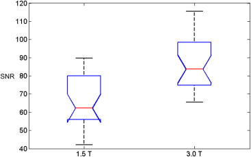
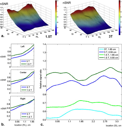
To identify the presence and extent of artifacts in prostate diffusion-weighted magnetic resonance imaging (DW-MRI) and discuss tradeoffs between imaging at 1.5 T (1.5 T) and 3.0 T (3.0 T). In addition, we aim to provide quantitative estimates of signal-to-noise ratios (SNRs) at both field strengths.
Materials and Methods
The institutional review board waived informed consent for this Health Insurance Portability and Accountability Act–compliant, retrospective study of 53 consecutive men who underwent 3.0 T endorectal DW-MRI and 53 consecutive men who underwent 1.5 T endorectal DW-MRI between October and December 2010. One radiologist and one physicist, blinded to patient characteristics, image acquisition parameters, and field strength, scored DW-MRI artifacts. On b = 0 images, SNR was measured as the ratio of the mean signal from a region of interest (ROI) at the level of the verumontanum (the “reference region”) to the standard deviation from the mean signal in an artifact-free ROI in the rectum.
Results
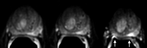
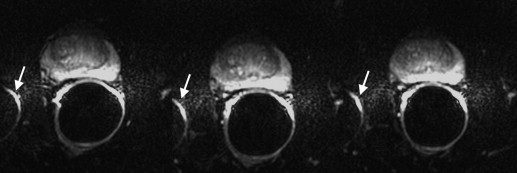
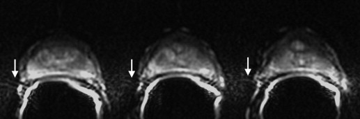
Both readers found geometric distortion and signal graininess significantly more often at 3.0 T than at 1.5 T ( P < .0001, all comparisons). Reader 2 (but not reader 1) found ghosting artifacts more often at 3.0 T ( P = .001) and blurring more often at 1.5 T ( P = .006). Mean SNR at the urethra (87.92 ± 27.76) at 3.0 T was 1.43 times higher than at 1.5 T (64.51 ± 14.96) ( P < .0001).
Conclusions
At 3.0 T (as compared to 1.5 T), increased SNR on prostate DW-MRI comes at the expense of geometric distortion and can also lead to more pronounced ghosting artifacts. Therefore, to take full advantage of the benefits of 3.0 T, further improvements in acquisition techniques are needed to address DW-MRI artifacts corresponding to higher field strengths.
Diffusion-weighted MR imaging (DW-MRI) is a promising technique that can provide both qualitative and quantitative information regarding the mobility of water molecules within tissue, can be added to existing imaging protocols without a substantial increase in the overall examination time (1–5 minutes), and does not require the administration of exogenous contrast material . Preliminary studies at both 1.5 T (T) and 3.0 T have suggested that DW-MRI may have clinical utility in the detection and management of prostate cancer. The recent trend is toward the use of 3.0 T clinical MRI scanners, under the premise of exploiting potential benefits of a higher signal-to-noise ratio (SNR).
DW-MRIs are most commonly collected using acquisition schemes based on the widely available single-shot spin-echo echo-planar imaging (SSSE-EPI) sequence, using a pair of rectangular-shaped gradient pulses along three orthogonal axes. The “snapshot” image acquisition methodology minimizes motion artifacts, hence minimizing the need for advanced postprocessing. However, SSSE-EPI is vulnerable to susceptibility-related image artifacts, which can have a detrimental effect on image quality and can interfere with diagnostic interpretation. Susceptibility artifacts occur near the interfaces of materials of different magnetic susceptibility, such as bone–soft tissue or air-tissue interfaces, as the result of microscopic gradients or frequency shifts. The artifacts that result from these local magnetic field inhomogeneities are spatial displacements of several pixels (ie, image distortion) and/or signal dropout. It has been suggested that susceptibility artifacts can increase exponentially with field strength , and they are known to cause significant geometric image distortions, stretching, and blurring on DW-MRIs at 3.0 T . Other limitations of EPI acquisition are the relatively low spatial resolution achievable with the present hardware and the inherently long echo-train, which lead to image blurring.
Get Radiology Tree app to read full this article<
Get Radiology Tree app to read full this article<
Get Radiology Tree app to read full this article<
Materials and methods
Get Radiology Tree app to read full this article<
Table 1
Distribution of Patient Characteristics
1.5 T 3.0 T_n_ %n % Biopsy Gleason grade 3 + 3 30 57 29 55 3 + 4 13 25 11 21 4 + 3 6 11 8 15 4 + 4 3 5 3 5 4 + 5 1 2 2 4
Median Range Median Range Age (years) 62 41–83 64 37–86 Prostate-specific antigen (ng/mL) 4.60 0.05–18.9 4.90 0.05–36.4
Get Radiology Tree app to read full this article<
MRI Data Acquisition
Get Radiology Tree app to read full this article<
Table 2
Distribution of Acquisition Parameters
Parameter 1.5 T 3.0 T Echo time 80.6 (72.4–89.8) ms 77.6 (69.6–101.2) ms Repetition time 3500 (2925–5075) ms 3500 (3300–6300) ms Field of view 140 mm 160 mm Matrix (frequency × phase) 96 × 96 128 × 128 Slice thickness 3 mm 3 mm Voxel size 1.46 × 1.46 × 3 mm 1.25 × 1.25 × 3 mm Acceleration factor 2 2 Pixel bandwidth 1304 Hz 1953 Hz
Get Radiology Tree app to read full this article<
Image Analysis
Get Radiology Tree app to read full this article<
Get Radiology Tree app to read full this article<
Table 3
Summary of Artifacts and Their Descriptions
Artifact Description Motion/ghosting Artifacts caused by patient or organ motion during acquisition of data creating ghost images in the phase-encode direction Image blurring Image blurring resulting from the low spatial resolution and long-echo train of the echo-planar imaging acquisition Susceptibility Artifacts that occur near the interfaces of materials of different magnetic susceptibility, manifesting as spatial displacement of several pixels and/or signal dropout Geometric distortion Distortions resulting from magnetic field inhomogeneity Signal “graininess” The presence of noise, which gives the image a mottled, grainy, textured, or snowy appearance (a qualitative measure of signal-to-noise ratio)
Get Radiology Tree app to read full this article<
Get Radiology Tree app to read full this article<
Get Radiology Tree app to read full this article<
Statistical Analysis
Get Radiology Tree app to read full this article<
Results
Get Radiology Tree app to read full this article<
Table 4
Comparison of Rates of Occurrence of Image Artifacts among 1.5 T and 3.0 T Diffusion-Weighted Magnetic Resonance Images According to Two Readers
Artifact Reader 1: Radiologist Reader 2: Physicist 1.5 T 3.0 T_P_ ∗ 1.5 T 3.0 T_P_ ∗ Motion/ghosting 86.8 (46) 96.2 (51) 0.1 (NS) 20.8 (11) 52.8 (28) .001 Blurring 18.9 (10) 24.5 (13) .5 (NS) 30.2 (16) 7.5 (4) .006 Susceptibility 7.5 (4) 3.8 (2) .3 (NS) 13.2 (7) 26.4 (14) .09 (NS) Geometric distortion 26.5 (14) 79.2 (42) <.0001 39.6 (21) 81.1 (43) <.0001 Signal “graininess” 75.5 (40) 9.4 (5) <.0001 58.5 (31) 13.2 (7) <.0001 Incorrect coil placement 5.7 (3) 1.9 (1) .6 (NS) 1.9 (1) 1.9 (1) 1.0 (NS)
NS, not significant.
The values represent the percentages of cases in which the readers indicated that the artifact was present, whereas the values in parentheses represent the actual numbers of cases in which each artifact was present out of a total of 53 patients in each group.
Get Radiology Tree app to read full this article<
Get Radiology Tree app to read full this article<
Get Radiology Tree app to read full this article<
Table 5
Comparison of the Locations of Area(s) Worst Affected by Artifacts on 1.5 T and 3.0 T Diffusion-Weighted Magnetic Resonance Imaging Studies as Determined by Each Reader
Artifact Reader 1: Radiologist Reader 2: Physicist 1.5 T 3.0 T_P_ ∗ 1.5 T 3.0 T_P_ ∗ None 5.7 (3) 13.2 (7) .1 (NS) 45.3 (24) 18.9 (10) .002 Seminal vesicles/base 66.0 (35) 81.1 (43) .1 (NS) 22.6 (12) 35.9 (19) .1 (NS) Midgland 7.5 (4) 11.2 (6) .1 (NS) 13.2 (7) 34.0 (18) .09 (NS) Apex 35.8 (19) 17.0 (9) .09 (NS) 34.0 (18) 21.0 (11) .5 (NS)
NS, not significant.
The readers selected from the following options: none, seminal vesicles/base, midgland, and apex. The values represent the percentages of cases where the readers indicated that the artifact was present, whereas the values in brackets represent the actual numbers of cases out of a total of 53 patients in each group.
Get Radiology Tree app to read full this article<
Get Radiology Tree app to read full this article<
Get Radiology Tree app to read full this article<
Get Radiology Tree app to read full this article<
Get Radiology Tree app to read full this article<
Get Radiology Tree app to read full this article<
Discussion
Get Radiology Tree app to read full this article<
Get Radiology Tree app to read full this article<
Get Radiology Tree app to read full this article<
Get Radiology Tree app to read full this article<
Get Radiology Tree app to read full this article<
Get Radiology Tree app to read full this article<
Get Radiology Tree app to read full this article<
Get Radiology Tree app to read full this article<
Get Radiology Tree app to read full this article<
Get Radiology Tree app to read full this article<
Acknowledgments
Get Radiology Tree app to read full this article<
Get Radiology Tree app to read full this article<
References
1. Koh D.M., Collins D.J.: Diffusion-weighted MRI in the body: applications and challenges in oncology. AJR Am J Roentgenol 2007; 188: pp. 1622-1635.
2. Issa B.: In vivo measurement of the apparent diffusion coefficient in normal and malignant prostatic tissues using echo-planar imaging. J Magn Reson Imaging 2002; 16: pp. 196-200.
3. Shimofusa R., Fujimoto H., Akamata H., et. al.: Diffusion-weighted imaging of prostate cancer. J Comp Assisted Tomogr 2005; 29: pp. 149-153.
4. Sato C., Naganawa S., Nakamura T., et. al.: Differentiation of noncancerous tissue and cancer lesions by apparent diffusion coefficient values in transition and peripheral zones of the prostate. J Magn Reson Imaging 2005; 21: pp. 258-262.
5. Hosseinzadeh K., Schwarz S.D.: Endorectal diffusion-weighted imaging in prostate cancer to differentiate malignant and benign peripheral zone tissue. J Magn Reson Imaging 2004; 20: pp. 654-661.
6. Gibbs P., Pickles M.D., Turnbull L.W.: Diffusion imaging of the prostate at 3.0 tesla. Invest Radiol 2006; 41: pp. 185-188.
7. Kim C.K., Park B.K., Han J.J., et. al.: Diffusion-weighted imaging of the prostate at 3 T for differentiation of malignant and benign tissue in transition and peripheral zones: preliminary results. J Comp Assisted Tomogr 2007; 31: pp. 449-454.
8. Vargas H.A., Akin O., Franiel T., et. al.: Diffusion-weighted endorectal MR imaging at 3 T for prostate cancer: tumor detection and assessment of aggressiveness. Radiology 2011; 259: pp. 775-784.
9. Kuhl C.K., Gieseke J., von Falkenhausen M., et. al.: Sensitivity encoding for diffusion-weighted MR imaging at 3.0 T: intraindividual comparative study. Radiology 2005; 234: pp. 517-526.
10. Gillard J.H., Papadakis N.G., Martin K., et. al.: MR diffusion tensor imaging of white matter tract disruption in stroke at 3 T. Br J Radiol 2001; 74: pp. 642-647.
11. Siegel R., Naishadham D., Jemal A.: Cancer statistics, 2012. CA Cancer J Clinicians 2012; 62: pp. 10-29.
12. Cooperberg M.R., Broering J.M., Carroll P.R.: Time trends and local variation in primary treatment of localized prostate cancer. J Clin Oncol 2010; 28: pp. 1117-1123.
13. Jemal A., Ward E., Thun M.: Declining death rates reflect progress against cancer. PLoS One 2010; 5: pp. e9584.
14. Hoeks C.M., Barentsz J.O., Hambrock T., et. al.: Prostate cancer: multiparametric MR imaging for detection, localization, and staging. Radiology 2011; 261: pp. 46-66.
15. Barentsz J.O., Richenberg J., Clements R., et. al.: ESUR prostate MR guidelines 2012. Eur Radiol 2012; 22: pp. 746-757.
16. Cornfeld D.M., Weinreb J.C.: MR imaging of the prostate: 1.5T versus 3T. Magn Reson Imaging Clin North Am 2007; 15: pp. 433-448. viii
17. Pruessmann K.P., Weiger M., Scheidegger M.B., et. al.: SENSE: sensitivity encoding for fast MRI. Magn Reson Med 1999; 42: pp. 952-962.
18. Sodickson D.K., Griswold M.A., Jakob P.M.: SMASH imaging. Magn Reson Imaging Clin North Am 1999; 7: pp. 237-254. vii-viii
19. Bammer R., Auer M., Keeling S.L., et. al.: Diffusion tensor imaging using single-shot SENSE-EPI. Magn Reson Med 2002; 48: pp. 128-136.
20. Noworolski S.M., Crane J.C., Vigneron D.B., et. al.: A clinical comparison of rigid and inflatable endorectal-coil probes for MRI and 3D MR spectroscopic imaging (MRSI) of the prostate. J Magn Reson Imaging 2008; 27: pp. 1077-1082.
21. Rosen Y., Bloch B.N., Lenkinski R.E., et. al.: 3T MR of the prostate: reducing susceptibility gradients by inflating the endorectal coil with a barium sulfate suspension. Magn Reson Med 2007; 57: pp. 898-904.
22. Brown J.J., Duncan J.R., Heiken J.P., et. al.: Perfluoroctylbromide as a gastrointestinal contrast agent for MR imaging: use with and without glucagon. Radiology 1991; 181: pp. 455-460.
23. Mitchell D.G., Vinitski S., Mohamed F.B., et. al.: Comparison of Kaopectate with barium for negative and positive enteric contrast at MR imaging. Radiology 1991; 181: pp. 475-480.
24. Panaccione J.L., Ros P.R., Torres G.M., et. al.: Rectal barium in pelvic MR imaging: initial results. J Magn Reson Imaging 1991; 1: pp. 605-607.