Image Browsing in Slow Medical Liquid Crystal Displays

Rationale and Objectives

Statistics show that radiologists are reading more studies than ever before, creating the challenge of interpreting an increasing number of images without compromising diagnostic performance. Stack-mode image display has the potential to allow radiologists to browse large three-dimensional (3D) datasets at refresh rates as high as 30 images/second. In this framework, the slow temporal response of liquid crystal displays (LCDs) can compromise the image quality when the images are browsed in a fast sequence.

Materials and Methods

In this article, we report on the effect of the LCD response time at different image browsing speeds based on the performance of a contrast-sensitive channelized-hoteling observer. A stack of simulated 3D clustered lumpy background images with a designer nodule to be detected is used. The effect of different browsing speeds is calculated with LCD temporal response measurements from our previous work. The image set is then analyzed by the model observer, which has been shown to predict human detection performance in Gaussian and non-Gaussian lumpy backgrounds. This methodology allows us to quantify the effect of slow temporal response of medical liquid crystal displays on the performance of the anthropomorphic observers.

Results

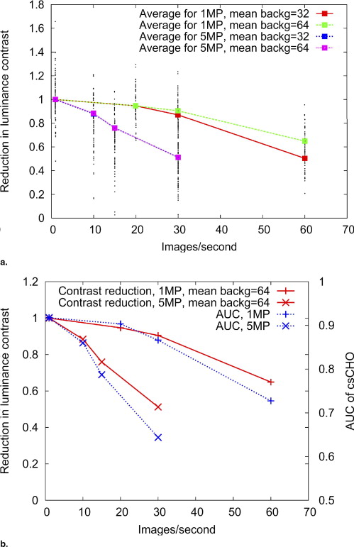
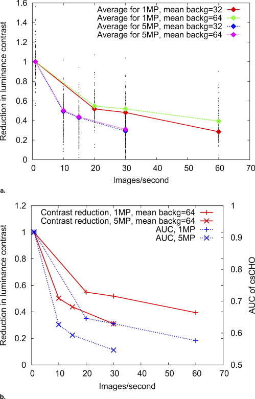
We find that the slow temporal response of the display device greatly affects lesion contrast and observer performance. A detectability decrease of more than 40% could be caused by the slow response of the display.

Conclusions

After validation with human observers, this methodology can be applied to more realistic background data with the goal of providing recommendations for the browsing speed of large volumetric image datasets (from computed tomography, magnetic resonance, or tomosynthesis) when read in stack-mode.

The high-fidelity display of medical images helps radiologists make correct diagnoses. Active-matrix liquid crystal displays (LCDs) are taking the place of traditional cathode-ray tube (CRT) displays and hard-copy films in most medical diagnostic imaging modalities. The image quality of LCD monitors has been significantly improved over the last few years. High-performance LCDs are considered to have comparable or better performance than CRTs in displaying static images for all aspects of display performances except noise and viewing angle ( ). However, LCDs can be inferior to CRTs at displaying moving scenes due to their slow response and the hold-type addressing scheme used in their pixel addressing methods ( ).

With the increasing number of computed tomography (CT) images to be interpreted per day, the ability of showing a fast sequence of images in stack-mode has been described as a preferred choice for a medical display. When using stack-mode browsing, slices are stacked on top of each other in the display memory buffer. At a given point, only one image is visible on the screen with the images being browsed back and forth at high image refresh rates under the control of the radiologist. When a high browsing speed is used, the radiologist perceives a three-dimensional (3D) volumetric image instead of a series of separate slices. The refresh rate could reach 30 images per second (ie, the duration for each specific image on the screen is only 33 milliseconds) depending on the application and equipment used ( ). Further increase of browsing speed with the advancement of technology is expected.

Get Radiology Tree app to read full this article<

Open full size image

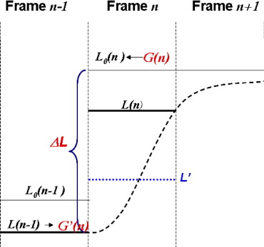
Figure 1

Luminance change for a dynamic scene. L 0 (i, j, n) indicates the target luminance of pixel ( i, j ) at frame n , corresponding to a gray level g 0 (i, j, n) . At frame n + 1 , the target gray level is g 0 (i, j, n + 1) (target luminance level L 0 (i, j, n + 1) ). Because of slow temporal response, the achieved luminance at frame n + 1 is L(i, j, n + 1) . The profile of luminance change from frame n to n + 1 may take different forms, as indicated by the dashed lines, depending on different liquid crystal display technologies and different gray level transitions.

Get Radiology Tree app to read full this article<

Materials and methods

Measurements

Get Radiology Tree app to read full this article<

Simulation of Temporal Effects

Get Radiology Tree app to read full this article<

g(r)=∑Kk=1∑Nkn=1b(1akn(r−rk−rkn),Rθkn) g

(

)

∑

(

−

)

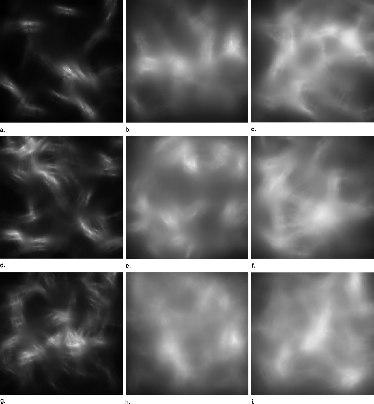
where r k represents position of the k th cluster, a kn represents scale of the n th blob within the k th cluster, θ kn is rotation angle of the n th blob within the k th cluster, and b(r,R θ ) is blob profile rotated at angle θ. To represent the power-law characteristics of the background, asymmetrical exponential blobs are used with characteristic length L x and L y in x and y directions. The details can be found elsewhere ( ). In this work, blobs and clusters are randomly distributed in a 3D cube to simulate 3D breast CT or tomosynthesis slices. Fifty independent 3D CLBs are generated for the temporal effect calculation. The mean number of clusters was set to be 160, and the mean number of blobs per cluster was set to be 20. The designer nodule is used as a signal to be detected ( ) and added to the center slice.

Get Radiology Tree app to read full this article<

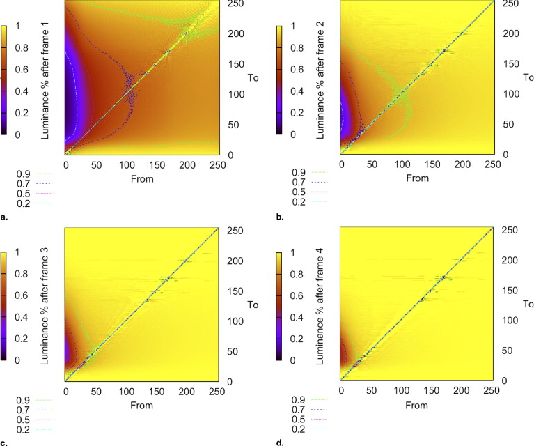
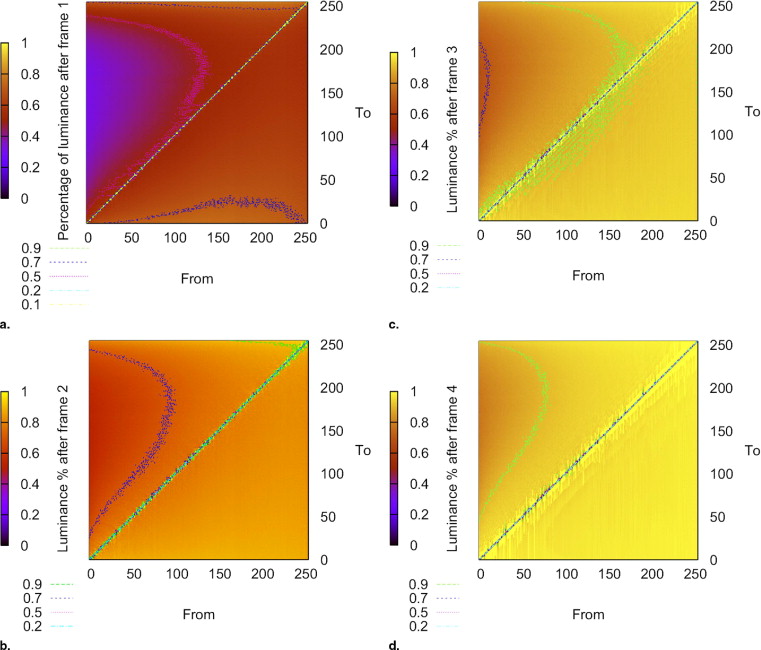
L(n)=L(n−1)+ΔL(g0(n),C−1(L(n−1)))*P(g0(n),C−1(L(n−1))) L

(

)

(

−

)

(

)

−

(

−

)

(

)

−

(

−

)

where g 0 (n) is the target gray level of pixel ( i, j ) at time index n, L(n − 1) is the achieved luminance level at the end of frame n−1 . The achieved gray level corresponding to an arbitrary screen luminance is calculated using the luminance response function of the device ( L = C(g) ). Because actual luminance values are mapped to a floating-point representation of the gray scale, we define C −1 (L) as its nearest integer value. Δ L(*) is the theoretical increase in luminance given by the grayscale calibration of the display device for the corresponding gray levels, and denotes the element-wise multiplication of matrix elements. For the next time index or frame, a similar equation can be written:

L(n+1)=L(n)+ΔL(g0(n+1),C−1(L(n)))*P(g0(n+1),C−1(L(n))) L

(

)

(

)

(

)

−

(

)

(

)

−

(

)

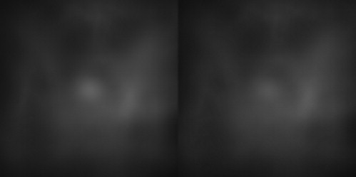
The change of luminance at pixel ( i,j ) is illustrated in Fig 3 . Note that the luminance level depends not only on the temporal characteristics of the display device, but also on the history of the pixel luminance. The calculations assume that luminance is constant in a frame time, shown as the horizontal thick lines in the graph. In reality it will take some time for the luminance to change from frame n −1 to n . The luminance may take different tracks depending on different transitions and display technology, as illustrated in Fig 1 for transition at frame n . We also consider the linear case to compare with the constant luminance case. The linear approximation assumes that the integrated luminance is a good estimate for the perceived luminance. Alternatively, a constant luminance model can also be used. By running the CLB slices through such an LCD temporal response model, images that represent actual displayed values on LCDs can be calculated. Figure 4 shows an example of our method to simulate temporal response effects on medical images.

Get Radiology Tree app to read full this article<

LC=Ls−LbLb L

−

where L s is the average luminance of the signal and L b is the average luminance of the background in the region adjacent to the signal. However, this metric doesn’t always correlate with detectability. To further quantify the effects of temporal response, a computational observer was used to estimate detectability under different browsing speeds.

Get Radiology Tree app to read full this article<

Results

Get Radiology Tree app to read full this article<

Discussion

Get Radiology Tree app to read full this article<

Conclusions

Get Radiology Tree app to read full this article<

Appendix

Computational model observer

Get Radiology Tree app to read full this article<

C(l¯)=1C0csf(μ,l¯) C

(

)

(

)

where μ is the frequency of the signal to be detected, ̄l is the mean luminance in a field of view (FOV) of an image, and csf(.) is the contrast sensitivity model of the human visual system. Then we use C(̄l) to determine if a pixel luminance is above the threshold:

lk−l¯l¯<C(l¯)→lk=l¯ l

−

(

)

→

where l k is the luminance of the k th pixel in the image. If the given relation is satisfied, the luminance of the kth pixel in the image is replaced by the mean luminance of the field of view; if not, the luminance of the k th pixel is left unchanged. Finally, the CHO with difference-of-Gaussian channels was applied to the resulting image. We fixed C at a value for which the csCHO matches human performance in one of the experiment conditions. Then we calculated the csCHO performance for the other experiments. csCHO has been shown to well predict human performance in detection tasks using lumpy backgrounds. More details on the performance of the csCHO will be presented in a separate article ( ).

Get Radiology Tree app to read full this article<

References

1. Badano A.: AAPM/RSNA tutorial on equipment selection: PACS equipment overview: display systems. Radiographics 2004; 24: pp. 879-889.
2. Tsukuda T.: TFT/LCD: liquid crystal displays addressed by thin film transistors.1996.Gordon and Breach Science PublishersAmsterdam, The Netherlands
3. Kurita T., Saito A., Yuyama I.: Consideration on perceived MTF of hold type display for moving images. Proc Int Display Workshop’98 1998; pp. 823-826.
4. Miseli J.: Motion artifacts. Proc SID 2004; pp. 86-89.
5. Mathie A.G., Strickland N.H.: Interpretation of CT scans with PACS image display in stack mode. Radiology 1997; 203: pp. 207-209.
6. Reiner B.I., Siegel E.L., Hooper F.J., et. al.: Radiologists productivity in the interpretation of CT scans: a comparison of PACS with conventional film. AJR Am J Roentgenol 2001; 176: pp. 861-864.
7. den Boer W.: Active Matrix liquid crystal displays: fundamentals and applications.2005.ElsevierBurlington, MA
8. Nakamura H., Crain J., Sekiya K.: Optimized active-matrix drives for liquid crystal displays. J Appl Phys 2001; 90: pp. 2122-2127.
9. Barrett H.H., Myers K.J.: Foundations of image science.2004.WileyHoboken, NJ
10. Park S., Gallas B.D., Badano A., et. al.: Efficiency of the human observer for detecting a gaussian signal at a known location in non-gaussian distributed lumpy backgrounds. J Optical Soc Am A Optics Image Sci Vision 2007; 24: pp. 911-921.
11. Myers K.J., Barrett H.H.: Addition of a channel mechanism to the ideal-observer model. J Opt Soc Am A 1987; 4: pp. 2447-2457.
12. Abbey C.K., Barrett H.H.: Human- and model-observer performance in ramp-spectrum noise: effects of regularization and object variability. J Opt Soc Am A 2001; 18: pp. 473-487.
13. Gallas D.B., Barrett H.H.: Validating the use of channels to estimate the ideal linear observer. J Opt Soc Am A 2003; 20: pp. 1725-1738.
14. Liang H., Badano A.: Precision of gray level response time measurements of medical liquid crystal display. Rev Scient Instr 2006; 77: pp. 065104.
15. Bochud F.O., Abbey C.K., Eckstein M.P.: Statistical texture synthesis of mammographic images with clustered lumpy backgrounds. Optic Exp 1999; 4: pp. 33-43.
16. Burgess E.A., Jacobson F.L., Judy P.F.: Human observer detection experiments with mammograms and power-law noise. Med Phys 2001; 28: pp. 419-437.
17. Barten P.G.J.: Contrast sensitivity of the human eye and its effects on image quality.1999.SPIE PressBellingham, WA
18. Eckstein M.P., Whiting J.S., Thomas J.P.: Role of knowledge in human visual temporal integration in spatiotemporal noise. J Opt Soc Am A 1996; 13: pp. 1960-1968.
19. Bartlett N.R.: Thresholds as dependent on some energy relations and characteristics of the subject.Graham C.H.Vision and visual perception.1965.WileyNew York:pp. 154-184.
20. Liang H., Badano A.: Temporal response of medical liquid crystal displays. Med Phys 2007; 34: pp. 639-646.
21. Park S, Badano A, Gallas BD, et al. A contrast-sensitive channelized observer. IEEE Trans Med Imaging. In press.

Image Browsing in Slow Medical Liquid Crystal Displays

Rationale and Objectives

Materials and Methods

Results

Conclusions

Materials and methods

Measurements

Simulation of Temporal Effects

Results

Discussion

Conclusions

Appendix

Computational model observer

References

Further Reading

30% unnecessary

Abstracts of Funded National Institutes of Health Grants

Audience Response Systems in Medical Student Education Benefit Learners and Presenters